Chapter 10
Using GAIA
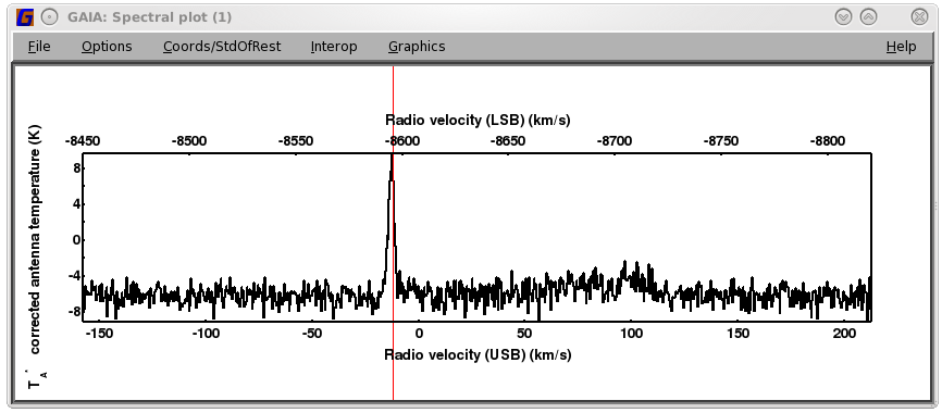
10.1 Removing a baseline with GAIA
-
(1)
- Select the spectrum you want to use as your template for the entire cube.
-
(2)
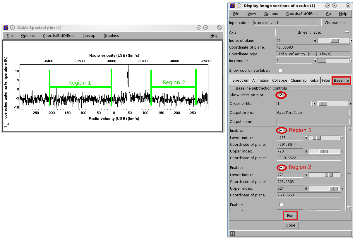
- Select the Baseline tab in the "
Display image sections
     of a cube
" window.
-
(3)
- Select the order of the baseline you want to fit and remove.
-
(4)
- Check the Show limits on plot button to interactively draw your baseline windows. You can click
and drag the edges of these limit lines in the "
Spectral plot" window.
-
(5)
- Check Enable for each new baseline window you want to define.
-
(6)
- Click Run.
10.2 Creating channel maps with GAIA
You can display channel maps in Gaia by selecting the region of a spectrum you wish to collapse over. You can
use a spectrum from any of the pixels in the cube and the region selected will be applied to the whole
map.
-
(1)
- Select the spectrum you want to use as your template for the entire cube.
-
(2)
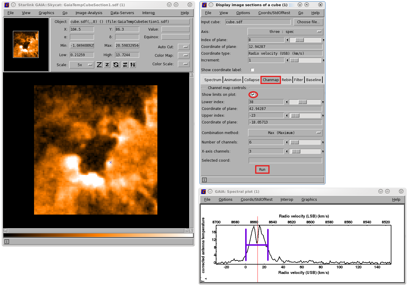
- Select the Chanmap tab in the "
Display image sections of a cube" window.
-
(3)
- Check the Show limits on plot box to interactively draw the range over which to collapse your
cube. You can click and drag the end-bars of the limit lines in the "
Spectral plot" window.
-
(4)
- Select the collapse method (Max is chosen in the example).
-
(5)
- Use the slider bars to select the total number of channels you want to generate and the number of
x-axis channels. The x-axis channel number sets the aspect ratio for the resulting display
grid.
-
(6)
- Click Run. The result is shown in the figure below.
10.3 Contouring with GAIA
-
(1)
- Open the map you wish to contour over.
-
(2)
- Select Image-AnalysisContouring
from the menu bar across the top of the main window.
-
(3)
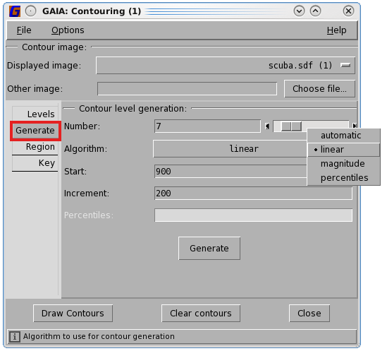
- Select the file you wish to contour in the "
Contouring" window.
-
(4)
- Generate your contours in the Generate tab found on the left-hand side of the "
Contouring"
window. The example below defines linearly spaced contours starting at 900K. Clicking the
Generate button will return you to the Levels tab.
You can also input or edit the contour levels manually in the Levels tab.
-
(5)
- Customise the look of your contours under the Options menu. You can experiment with the other tabs
(Region and Key) for options concerning contour area and legend.
-
(6)
- Click the Draw Contours button to make the contours appear over your map in the main window. If you
are contouring over a cube you can scroll through the velocity axis whilst the contours remain fixed on
top.
-
(7)
- To add a second set of contours select FileNew
window in the top menu of the "
Contouring" window. Here you can define a second image to be
contoured and specify new levels and appearance. Open as many new contouring windows as
necessary.
To save the graphic, there is a File
Print, but some people prefer a tool with a capture facility such as xv.
10.4 Overlaying clumps and catalogues with GAIA
Gaia can display two- or three-dimensional clump catalogues that have been generated by the Cupid routine
findclumps (see Section 9.5). Clump catalogues in this format are also available for download from the JCMT
Science Archive.
-
(1)
- Open your cube for three-dimensional clump finding or your integrated map for two-dimensional
clump finding.
-
(2)
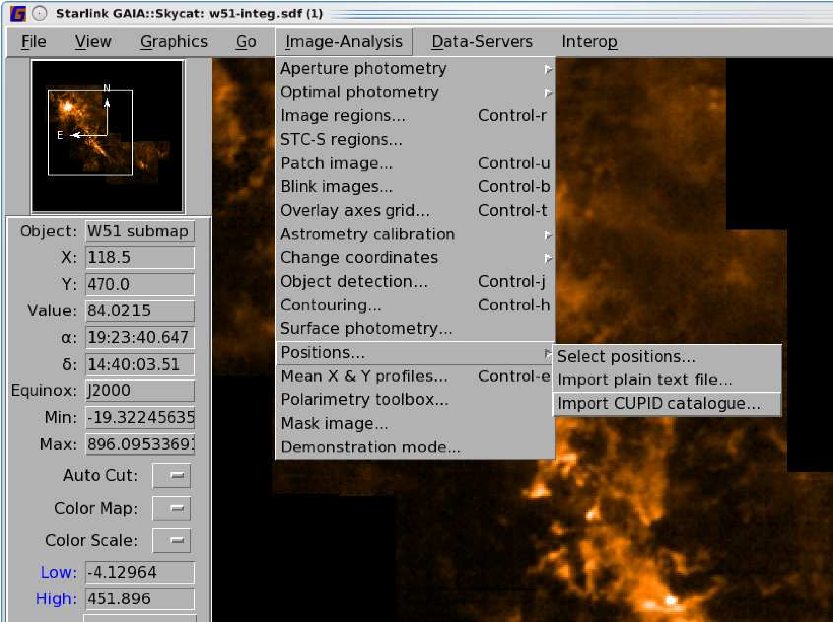
- Select Image-AnalysisPositionsImport
CUPID catalogue from the menu bar across the top of the main window. Note that for two-dimensional
catalogues an alternative route is to select Data-ServersLocal
catalogs. In this case you can skip Step 3.
-
(3)
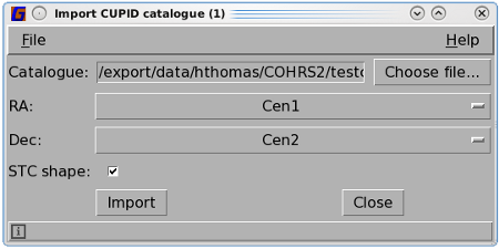
- In the "
Import CUPID catalogue" window, select a file with the Choose file... button. For polygon shapes
tick the STC shape box. You can change the RA/Dec co-ordinates from Cen1/Cen2, which give the
central position of the clumps, to Peak1/Peak2 which give the position of the peak within
them.
-
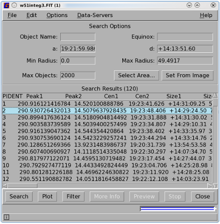
(4)
- A catalogue window for your FITS file will appear listing all the sources and their positions and
extents.
-
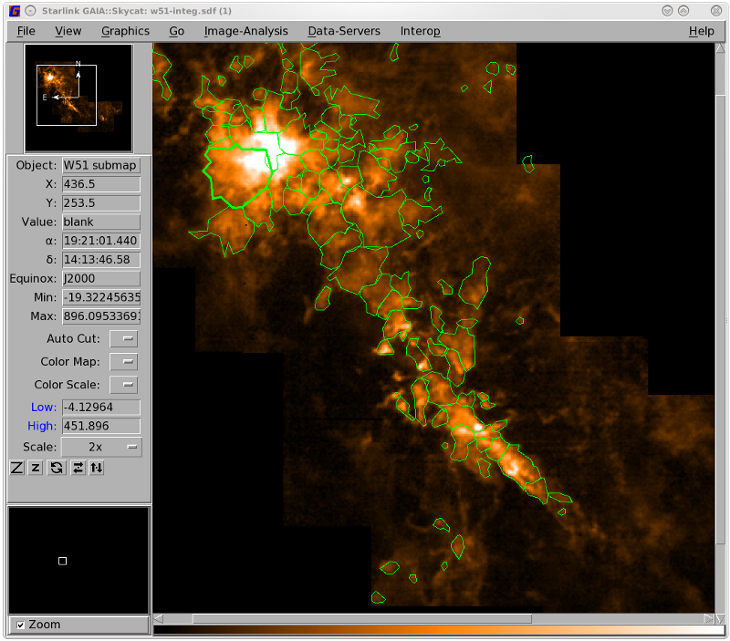
(5)
- Outlines of your clumps, or symbols at the peak positions, will be automatically overlaid on
your map. If this does not happen, click the Plot button on the catalogue window. When you
click on a clump from the catalogue list the outline of that clump will appear in bold on your
map.
-
(6)
- If you are displaying a three-dimensional catalogue over a cube, it will only display clumps which
include data from the current slice. The clumps shown will update as you move through the
cube.
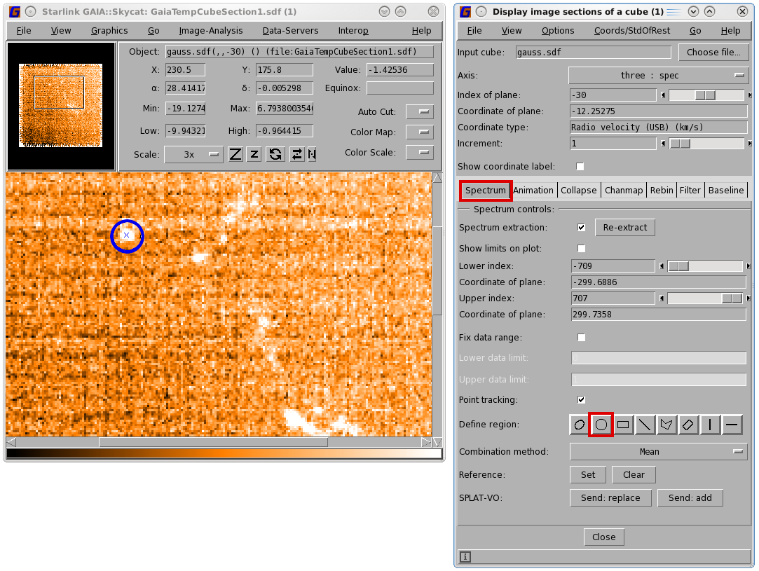
10.5 Displaying average spectrum with GAIA
-
(1)
- Select the Spectrum tab in the "
Display image sections of a cube" window.
-
(2)
- Define the shape of your region by selecting one of the Define region buttons (a circle is chosen in
the example below).
-
(3)
- Select the combination method (Mean is chosen in the example below).
-
(4)
- Draw the shape on your map by clicking and dragging the mouse. The "
Spectral plot" window will
automatically update to show your combined spectrum. You can re-position and resize your shape at any
time. You can see from Figure 10.12 that the averaged spectrum gives a much clearer profile of the
source.
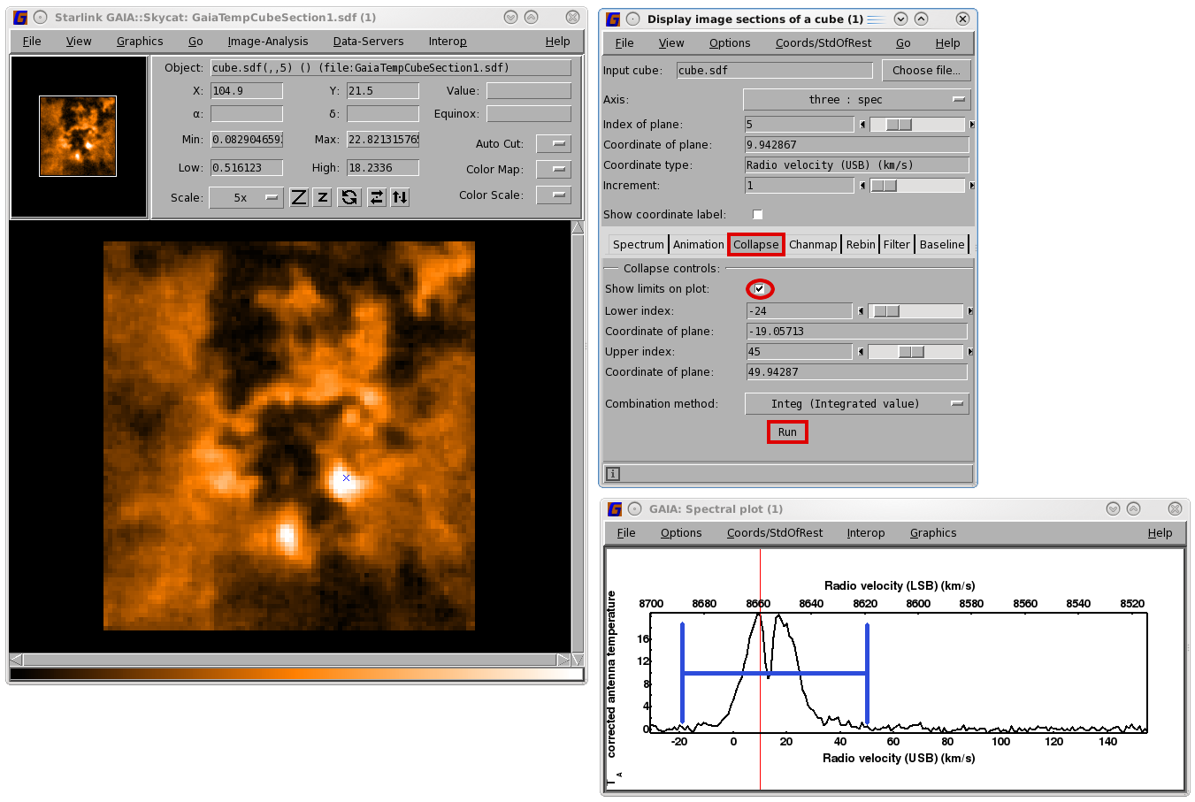
10.6 Collapsing your cube with GAIA
-
(1)
- Select the axis you want to collapse you to collapse over by selecting from the Axis drop-down list
in the "
Display image sections of a cube" window.
-
(2)
- Select the spectrum you want to use as a template for your cube.
-
(3)
- Select the Collapse tab in the "
Display image sections of a cube" window.
-
(4)
- Check the Show limits on plot button to interactively select your collapse region. You can click
and drag the edges of these limit lines in the "
Spectral plot" window. Position these around the
region you wish to collapse over.
-
(5)
- Select the collapse method via the Combination method drop-down list (Integ is selected in the
example below).
-
(6)
- Click Run. The main window will automatically update to show your collapse image.
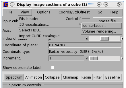
10.7 Three-dimensional visualisation with GAIA
-
(1)
- Select View3D
VisualisationIso
surfaces.../Volume rendering in the "
Display image sections of a cube" window.
-
(2)
- Click and drag the image display to change the orientation in the "
Volume render" window.
-
(3)
- Include axes labelling, the image plane and other features using the check boxes on the side
bar.
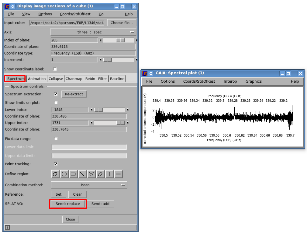
10.8 Sending spectra to SPLAT
Gaia has very limited analysis functionality for spectra. Whereas Splat is a sophisticated graphical
spectral-analysis tool. Any spectrum displayed in Gaia (a single-position spectrum or a spectrum averaged
over some region 10.5) can be sent (via a protocol called SAMP) to Splat for more-detailed spectral
analysis.
Splat offers the ability to further process, fit, or identify spectral lines. You can also plot different spectra in
the same window and make publishable files. The full Splat documentation can be found here in
SUN/243.
Here are some instructions on how to do this.
-
(1)
- Start Splat, if it is not already running.
-
(2)
- Click on the Interop menu item in Splat. If the SAMP control icon has a red circle, it means that the SAMP
communication hub is running. If, however, the icon has a white circle, you need to start a hub. To do this
press the Register with HUB button at the bottom of the window, and then press the Start internal hub
button in the window that pops up.
-
(3)
- If you had Gaia already running before the hub was active, then in Gaia select the
InteropRegister
to register your GAIA with the hub.
-
(4)
- Select the spectrum you wish to send from Gaia.
-
(5)
- Click on SPLAT-VO Send: replace or Send: add button near the bottom of the "
Display image sections
of a cube" window. The spectrum should appear in a Splat window.
SAMP can also transmit images and catalogues between compliant applications. For example, you might have a
selected catalogue of sources observed elsewhere in Topcat and want to plot the locations over your HARP
maps in Gaia.
Copyright © 2015-2021 Science and Technology Facilities Council,
& East Asian Observatory