Chapter 5
Running makemap Outside the Pipeline

The previous chapter described how to make maps using the SCUBA-2 Pipeline. Users—particularly new users—are encouraged to use the pipeline for their map-making. However, greater control of the map-making process is available by running the makemap command directly, rather than from within the pipeline. This chapter describes how to do this, but should be seen as “advanced usage”.

5.1 Running makemap

Before running makemap directly, you need to ensure that the Starlink environment has been initialised and the Smurf package started (see Section 1.3.2 and Section 1.3.3).

To run makemap, you need to supply values for the following command-line parameters¹:

If any of the above parameters are not given on the makemap command line, prompts will be issued and you will be invited to supply values for the missing parameters.

So an example command line would be:

Here, the file myfiles.lis contains a list of the raw data files to be included in the map, and could for instance look like this:

This uses all available data for all four 850 $\mu$m sub-arrays, for observation 30 taken on 20th July 2012².

The file dimmconfig_bright_compact is one of the pre-defined configuration files supplied with Smurf. It contains configuration parameter values that are optimised for creating maps from bright compact sources.

After the makemap command completes, the final map will be left in file 850_crl2688.sdf and can be displayed using Gaia:

There are many other command-line parameters that can be supplied when running makemap, but only the three listed above are mandatory. All the others assume default values if not supplied on the command-line. For a full list of all available command-line parameters, their functions and default values, see the description of makemap within the smurf document, SUN/258.

You can supply values for any of these extra parameters on the command line. For instance, one of the command-line parameters that is usually defaulted is PIXSIZE, which specifies the pixel size for the final map, in arcseconds. The default pixel sizes, defined as one quarter of the Airy disk rounded up to the nearest half arcsecond, are:

• 2 arcsec at 450$\mu$m
• 4 arcsec at 850$\mu$m

So for instance, the above command-line could be modified as follows to produce a map with 3-arcsecond pixels:

Note, if parameters are specified by name on the command-line, as in these examples, then the order in which they are specified is insignificant³. Also, parameter names are case-insensitive.

5.2 Interpreting the screen output from makemap

Whilst makemap runs, it outputs information continuously to the screen about what it is doing. The amount of information displayed can be controlled using the MSG_FILTER command-line parameter. It defaults to “normal”, but if you want more information you could set it to (say) “verbose”:

Note—unambiguous abbreviations may be used for many command line parameters—so “verb” is acceptable instead of “verbose”. Setting MSG_FILTER to “quiet” will suppress all screen output.

The following shows the screen output generated by a typical run of makemap if MSG_FILTER is left set to its default value of “normal”. Explanatory comments, which are not actually part of the output generated by makemap, are included in emphasised type. The input data are a short observation of a bright compact source (CRL 2688):

The output starts by reporting information about the input data files, including the number that contain on-sky bolometer values (“science” data), the astronomical object and the SCUBA-2 observation number.

Next comes information about the output map. The world coordinate system is described by means of the equivalent FITS-WCS keywords⁴

The reported pixel bounds of the output map refer to a pixel coordinate system in which the source is centred at position (0,0). Note, the definition of pixel coordinates within the NDF format allows the origin of pixel coordinates to be at any nominated position within the array—it does not have to be at the bottom left corner as in FITS—and makemap chooses to put the pixel origin at the specified source position.

Finally, the bounds of the map are given in the celestial coordinate system specified by the SYSTEM command-line parameter. This parameter defaults to “tracking”, which causes the map to be created in the celestial coordinate system in which the observation parameters were originally defined. It may instead be set to a specific coordinate system (e.g. “galactic”, “icrs”, etc.) to force the map to be made in that system.

By default, the data are down-sampled so that the on-sky distance between adjacent samples is roughly equal to the pixel size (4 arcseconds in this case). This saves memory and computing time without adversely affecting the final map. The degree of down-sampling can be controlled using the downsampscale configuration parameter.

Next comes information about the stopping criteria for the iterative map-making algorithm. In this case, iterations will stop when 40 iterations are completed, or the normalised change in the map between iterations reduces to less that 0.05. These values are specified by configuration parameters numiter and maptol (see Section 3.4).

In almost all cases, the raw data files constituting a SCUBA-2 observation will correspond to a single continuous stream of data samples, taken at roughly 200 Hz. Sometimes however, this may not be the case⁵, so you are now told how many chunks of data were found, and how long they were. Something may be wrong if the input data contains any breaks.

Next comes information about the amount of memory needed to make the map. If insufficient memory is available to process all the input data together, it will be split into chunks, and a separate map made from each chunk. These maps are later co-added to form the final output map. This can often result in a poorer map—see Data Chunking).

Finally, a loop is entered to process each chunk in turn, and you are told which chunk is currently being processed. In this case there is only one chunk (which is good).

We now start the first iteration of the iterative algorithm described in Section 3.2, to create a map from the current chunk of input data. We will be performing —- at most—40 iterations, as set by numiter.

Now we have a number of statistics describing the cleaned data prior to the first iteration⁶.

Each sub-array contains a grid of $32\times 40$ bolometers, making 5120 bolometers in total over all four sub-arrays. The number of time slices in the concatenated data after down-sampling is reported. In this case, 5957 time slices over 2.6 minutes, equating to a down-sampled frequency of about 38 Hz. The total number of samples is the product of the number of bolometers and the number of time slices. Each of the following lines indicates the percentage of the data that has been flagged as unusable for various reasons:

• BADDA – flagged as unusable during data acquisition.
• DCJUMP – flagged as unusable because of a sudden step change in the base-line.
• STAT – flagged as unusable because the telescope was stationary (or at least moving too slowly).
• NOISE – flagged as unusable because they were too noisy.

The BADBOL item gives the fraction of bolometers that have been flagged as entirely bad for any of these reasons, and from which no data will be used.

Indicates the models that are being calculated. More information about each individual model is displayed if you set MSG_FILTER=verbose on the makemap command line.

More statistics are displayed once the first iteration is completed and the first estimate of the science map has been generated. Data samples may be flagged as bad within the iterative stage for various reasons, and so these statistics may be different to those shown prior to the start of the iterative stage. Most significantly, the COM: line shows the percentage of data that has been rejected because the time stream did not resemble the common-mode signal closely enough. The “NORMALIZED MAP CHANGE” values are of no real significance on the first iteration since there is no previous map with which to compare the new map (in fact the numerical values are generated by comparing the new map with a map full of zeros).

The second iteration starts, and proceeds in much the same way as the first iteration. The main difference is that the NOI model is generated at the start of the second iteration. This model measures the variance within each bolometer time-stream. It is used to weight the bolometer samples when forming the mean sample value in each map pixel⁷. NOI is calculated from the residuals left after removal of all other models, and is only calculated once—subsequent iterations re-use the same NOI values.

The SPIKE: item that has appeared in the quality flagging statistics records the number of samples that have been rejected as transient spikes in the time-series. This flagging is done by comparing the bolometer values that fall in each map pixel, and flagging any that appear to be statistical outliers—see configuration parameter ast.mapspike.

The mean “NORMALIZED MAP CHANGE” value should drop with each subsequent iteration (note, the “max” normalised map change value can usually be ignored as it records the maximum normalised change in any single map pixel and is thus highly subject to random variations).

The mean normalised map change continues to drop with the third iteration, as expected. The total number of samples going into the map is dropping with each iteration, but only very slowly. This is mainly due to the increased number of samples being flagged by the COM model, but is at an acceptably small level.

After the fourth iteration the mean normalised map change has dropped to 0.0401588, which is below the value of 0.05 provided for the maptol parameter by the dimmconfig_bright_compact configuration file⁸. Consequently, makemap considers the map to have converged. However, in view of the fact that the dimmconfig_bright_compact configuration file uses “AST masking” (see Section 3.5.1), it is necessary to do one final iteration in order to assign correct values to the pixels that lie outside the source mask. Note, when AST masking is being used, the reported normalised map change values only include pixels that are within the source mask.

After the extra iteration required by AST masking has been performed, the final output map is created. It is always advisable to check the final number of samples available for the map, as a low value will cause your map to have high noise levels. In this case, 62.86% of the samples are available for the map, which is quite acceptable—only a couple of percent of the samples have been rejected by the map-making, mostly flagged by the COM model. The bulk of the bad samples (35.43%) were rejected during data acquisition due to dead bolometers etc.

Note, the numiter parameter is set to -40 by dimmconfig_bright_compact, meaning that no more than 40 iterations will be performed. In this particular case we only needed 4 iterations (plus a mandatory extra iteration) to achieve our requested maptol value. But it is possible for some observations—particularly observations of extended sources—to require more than 40 iterations to converge to a maptol of 0.05. In such cases the screen output will end with a message saying that the solution “FAILED TO CONVERGE”⁹. In such cases, you could simply increase numiter and re-run makemap, but you may also want to investigate the cause of the slow convergence using one or more of the techniques described in Chapter 9, as it may indicate some issue with the raw data.

Map pixels that receive a very small number of samples are automatically set bad. These are usually the pixels around the periphery of the observation, and will have very unreliable variance estimates. The threshold is determined by the hitslimit parameter, which defaults to 1 percent of the mean number of hits per pixel, corresponding to 4 samples per pixel in this case.

The observation used in this particular case was a short observation of a calibrator, lasting only 2.6 minutes. Consequently there was no need to divide the data up into multiple chunks in order to fit it into memory. However, for very long observations, or for shorter observations when using a computer with less than the recommended amount of memory (see Section 1.2), it may be necessary to process the raw data in multiple chunks. If this happens, a map is created from each chunk in turn, and all these maps are then added together to form the final map. The final message “Total samples available from all chunks: 19172853 (3218.54 bolos)” indicates the total number of samples (and equivalent number of bolometers) used from all chunks. In this case there was only one chunk, so these values are equal to the numbers reported at the end of the last iteration. Chunking often results in a poorer map and should be avoided if possible—see Data Chunking).

5.3 Interacting with makemap during a long run

For long observations, makemap can take several hours to run, particularly on slow or low-memory computers. For this reason it is useful to be able to monitor progress so that potential problems can be detected early, in order to avoid wasting time.

5.3.1 Monitoring screen output

The most straight-forward way of monitoring progress is to check the values written to the screen by makemap at the end of each iteration (see the previous section). For instance, if you run makemap as follows:

then the messages displayed by makemap on the screen will also be written to text file makemap.log. This makes it easy to search the log file whilst makemap is still running, for instance from another terminal window:

This displays the normalised change in maps between successive iterations, for the iterations that have so far been completed. If the mean normalised map change is not decreasing smoothly, (for instance if it is oscillating around a fixed value), then there is a potential problem. In which case you may want to interrupt the makemap process, rather than waiting potentially for several hours just to end up with a bad map.

Likewise, it is useful to monitor the total number of samples that are being pasted into the map at the end of each iteration:

The lower the percentage of samples included in the map, the greater will be the noise in the map. If this number drops much below 50% then you may want to think about aborting makemap and investigating why the number is so low (e.g. by looking at the “quality statistics” displayed at the end of each iteration, to determine the cause of the data loss).

Likewise, information can be gathered about chunking:

This indicates that the raw data has gaps in it, resulting in seven maps being made, one from each continuous chunk, before the final map is made by combining all the individual maps. Chunking can produce sub-optimal maps, and should normally be investigated—see Data Chunking.

5.3.2 Monitoring the map at the end of each iteration

The map created at the end of each iteration is normally discarded, but can be saved by setting configuration parameter itermap to either 1 or 2. By default, these “itermaps” are written to an extension of the main output NDF as described in Section 6.2, and cannot be viewed until makemap has completed. However, an alternative destination for these itermaps can be specified on the makemap command-line as follows, allowing them to be viewed whilst makemap is still running:

Note the distinction between the “itermaps” (plural) command-line option, and the “itermap” (singular) configuration parameter. As soon as the first iteration has finished, the above command will create a new file called myitermaps.sdf in which each itermap will be stored as soon as it is created. The file is closed after each itermap is written, and re-opened again before writing the next itermap. This is an example of a container file, where a single .sdf file contains several NDFs, each holding a different map (see Section 1.3.1). You can list the maps in such a file using Kappa ndfecho as follows:

The name of each itermap is of the form “CHxxIyyy”, where “xx” is the chunk number and “yyy” is the iteration number. In the common case where all raw data are processed in a single chunk, “xx” will be “00” for all itermaps.

You can view a single itermap using:

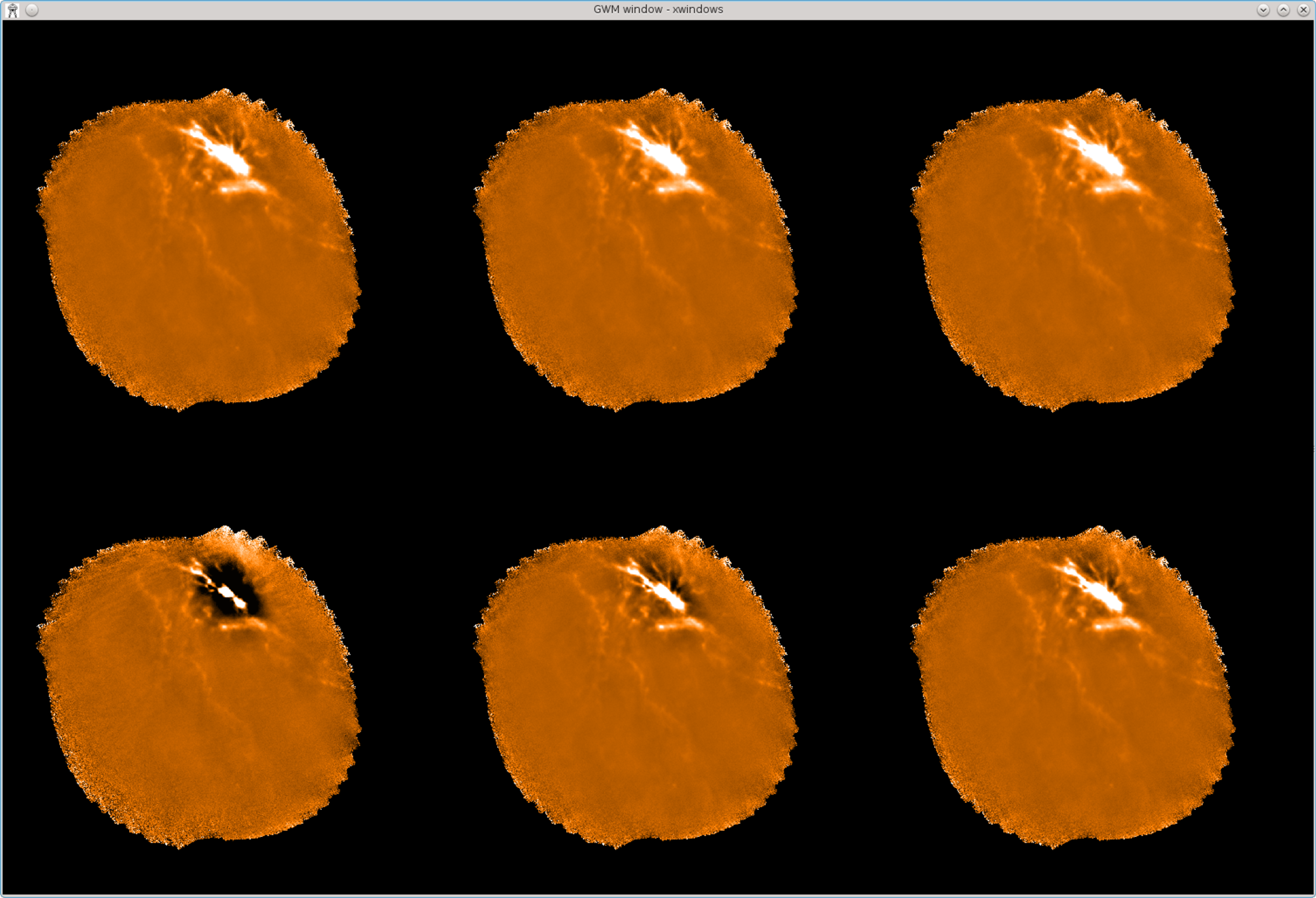
If you want to view several itermaps side-by-side, you can use Kappa picgrid to divide the screen up into a grid of “pictures”, then use picsel to pick each picture in turn, and use display to display an itermap in each one. For instance to display the first six itermaps side-by-side in a $3\times 2$ grid, all with the same scaling, without any axes, do:

This produces the display shown in Figure 5.1. Kappa display has many options for controlling things like data scaling, axis annotation and style, colour table, graphics device, etc..

Figure 5.1: The maps created on the first six iterations of makemap, from an observation of Orion A, using the dimmconfig_jsa_generic.lis configuration file with the addition of “itermap=1”. The first map is bottom left, and the sixth map is top right. This illustrates the initial fast improvement in the map over the first few iterations.

Alternatively, you can combine the itermaps into a 3D cube, and then use the cube-viewing facilities of Gaia to scroll through the itermaps in the style of a movie (see Section 6.2)¹⁰:

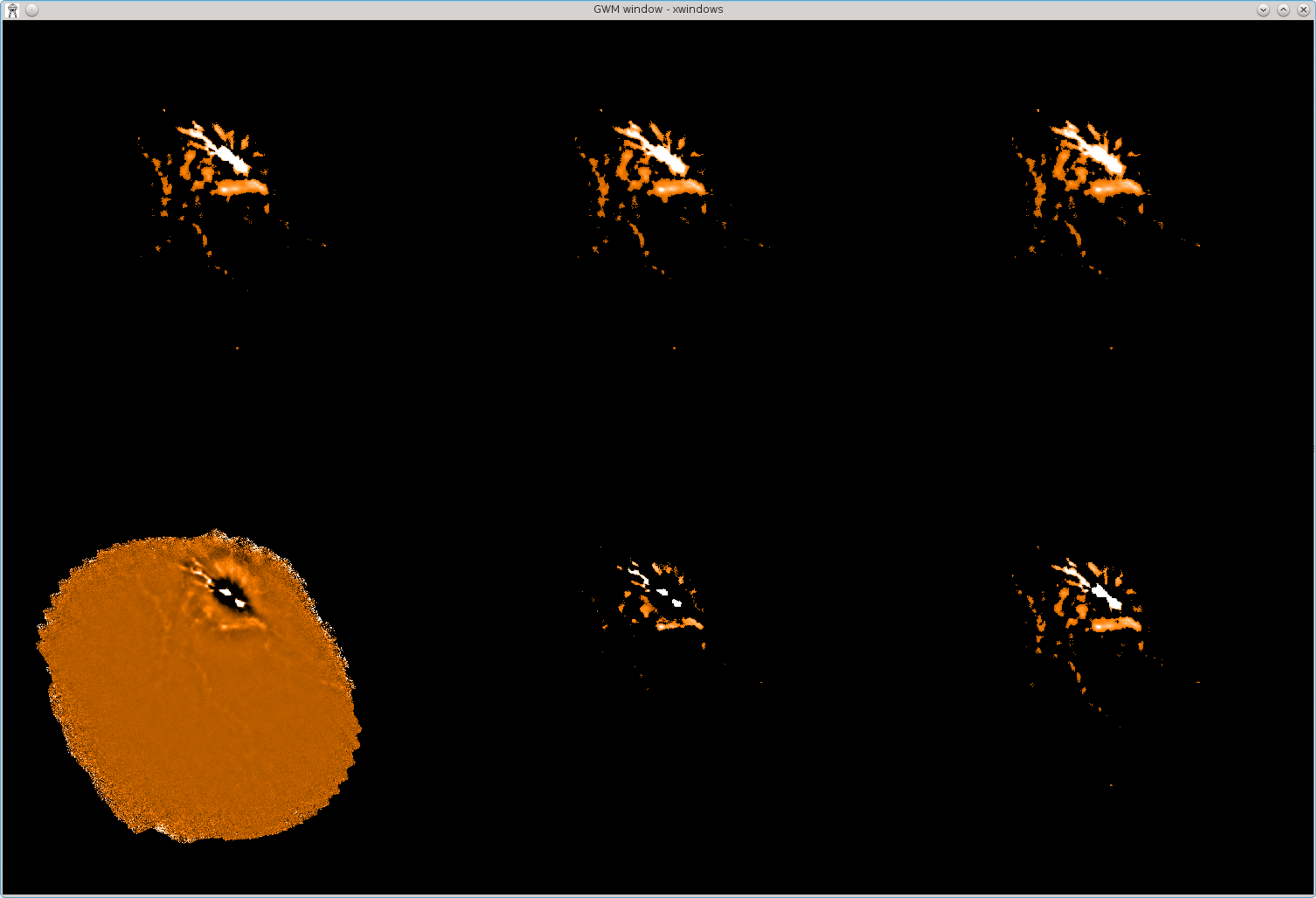
It is sometimes informative to look at the change between itermaps, to see the incremental effect of each iteration. This is most easily done if the itermaps are first stacked into a cube as described above. The next step is to produce a copy of the cube in which the pixel origin is moved by one pixel along the third axis (i.e. the axis that enumerates iteration). Finally subtract one cube from the other, and display the resulting difference cube (this example shows how command-line parameters can often be specified by position instead of by name when running Kappa commands—check the help information for each command to see the order in which options should be supplied):

This produces the display shown in Figure 5.2.

Figure 5.2: The difference between each pair of adjacent maps shown in Figure 5.1.

Viewing the mask after each iteration:

The above plots are based on the itermaps that are created by adding “itermaps=1” to your makemap configuration. You can instead use “itermaps=2”, which causes each itermap to be masked so that pixels outside the current source mask are set bad (i.e. blank)¹¹. Figure 5.3 shows the resulting itermaps.

Figure 5.3: The first six itermaps, create by using itermap=2 in the configuration. This causes pixels outside the source mask to be set blank, allowing the evolution off the mask to be seen (the first iteration is not masked). In this case, the mask includes all pixels above a signal-to-noise ratio of five.

The main point of this section is to emphasise that all the above investigations can be performed whilst makemap is still running, if you specify an explicit file for the itermaps using the “itermaps command-line option. This allows you to decide if the reduction is progressing as expected, and whether to interrupt the reduction.

5.3.3 Interrupting makemap

If you interrupt makemap by pressing control-C on the keyboard (or equivalently by sending an INT signal to the makemap process), it will continue until the current iteration is completed and then will issue a prompt with options allowing you to save the current map before closing, as in the following example:

<press control-C>

At this point you should respond to the prompt for parameter INTOPTION by typing 1, 2 or 3 followed by <return>. Option 1 aborts the process with an error status. Option 2 causes makemap to tidy up its internals and create a map from the current models just as if the iterative process had reached convergence. Option 3 causes one further iteration to be performed, without masking before creating a final map (you should use this option if you have been using AST masking—see Section 3.5.1).

5.4 Tips and tricks

5.4.1 Aligning your map with a pre-existing image

If you want to compare SCUBA-2 data with a map of the same region taken with a different instrument, you will usually want to create the SCUBA-2 map using the same pixel grid as the other map so that you can compare pixel values directly in the two maps¹². You can use the REF command-line parameter to do this. For instance, if your other map is in file herschel.sdf, you can do:

This will cause the output map in file outmap.sdf to use the same pixel grid as herschel.sdf. This means that a given point on the sky will have the same pixel coordinates in both maps, and so for instance you could divide one by the other to get a ratio map without any further alignment step:

This will divide outmap.sdf by herschel.sdf and put the ratio in ratio_map.sdf¹³.

However, by default makemap will trim the output map to exclude blank borders, thus the two maps may have different dimensions. NDF-based applications such as Kappa div automatically take account of this when comparing corresponding pixels in two NDFs—see Figure 5.4.

Figure 5.4: The curved dotted line represents a contour of an astronomical object. The heavy black lines represent the X and Y axes of the pixel coordinate system, crossing at the pixel origin (pixel_x,pixel_y)=(0,0). The numerical values represent pixel X and Y values. The blue box represents the bounds of the reference map supplied when running makemap. The red box represents the bounds of the map created by makemap. The reference image and the output image share the same pixel coordinate system, so a given point on the sky has the same pixel coordinates in both images. However, the output (red) image is cropped to remove blank borders and so has smaller dimensions than the reference (blue) image. All this is made possible by the fact that the NDF format, unlike FITS, does not require the origin of pixel coordinates to be at the bottom left corner of each map. NDF applications account for any difference in pixel origin when comparing pixels in different files.

If you want to force the output map to have certain bounds in pixel coordinates, you can do so by assigning values to the LBND and UBND parameters when running makemap. For instance, if you want to force the output map to have the same dimensions as the reference map, you could use Kappa ndftrace to list the properties of the reference NDF, including its pixel bounds, and then assign these bounds to LBND and UBND parameters when running makemap:

The resulting map in outmap.sdf will have the same pixel bounds as hershel.sdf.

5.4.2 Limiting the amount of memory used by makemap

There may be occasions when you need to limit the amount of memory used by makemap–for instance to leave enough memory for other processes to function correctly. For machines with more than 20 GB of memory, the default is to leave 4 GB free for other processes. For machines with less than than 20 GB of memory, the default is to leave 20% of the total memory free. This default can be over-ridden by indicating the maximum amount of memory that makemap should use by setting a value for the command-line parameter MAXMEM. For instance:

will ensure that makemap never uses more than 50000 MiB¹⁴ of memory. Be aware though that for larger observations this may cause the data to be processed in multiple chunks rather than a single continuous chunk, resulting in a poorer map.

5.4.3 Re-using previously cleaned data to speed up map-making

Usually, you will create your SCUBA-2 maps using one of the standard configuration files distributed with smurf (see Section 3.7). However, for certain problematic observations it may sometimes be necessary to experiment with several different configurations to find one that produces an acceptable map. In such cases a significant amount of time can be saved by re-using pre-cleaned raw data each time you make a map, rather than re-cleaning it each time.

By default makemap assumes that the supplied data are raw data that require cleaning before being used to make a map. However, if you include “doclean = 0” in your configuration, then makemap will skip the entire cleaning process and move directly on to the iterative map-making stage, thus saving significant time.

Obviously though, in this case you need to make sure that the data you supply to makemap have already been cleaned. There are two ways to get cleaned data:

(1)

You can run makemap initially on the un-cleaned data (i.e. the original raw data), and force makemap to dump the cleaned data to disk before going onto the iterative map-making stage. You can then re-use this cleaned data in subsequent invocations of makemap. To dump the cleaned data, you need to add “exportclean = 1” to the configuration on your initial run of makemap—don’t forget to remove it for subsequent runs! The cleaned data are put into files in the current directory, one for each sub-array, with names such as s8c20120706_00037_0003_con_res_cln.sdf. Note the _cln on the end of the name indicating cleaned data. The base name, “s8c20120706_00037_0003” in this case, is taken from the first raw data file that contributes to each chunk. If the entire observation is processed in one chunk (as it should usually be) then there will be one such _cln file for each sub-array. If the observation is split into multiple chunks, then there will be multiple _cln files for each sub-array (one for each chunk).

(2)

You can use the separate Smurf task sc2clean to clean the data as described in Appendix A.