Chapter 3
POL-2 Data Reduction – The Theory
3.1 The data flow
POL-2 data reduction is an involved process. A broad overview of this process is presented here first, followed
by a discussion of the specific details. It should be noted that this same procedure is used irrespective of
whether single or multiple observations are to be reduced.
The following description assumes that the makemap command is being used to create maps. Section 3.3
explains the effects of using the skyloop command in place of makemap.
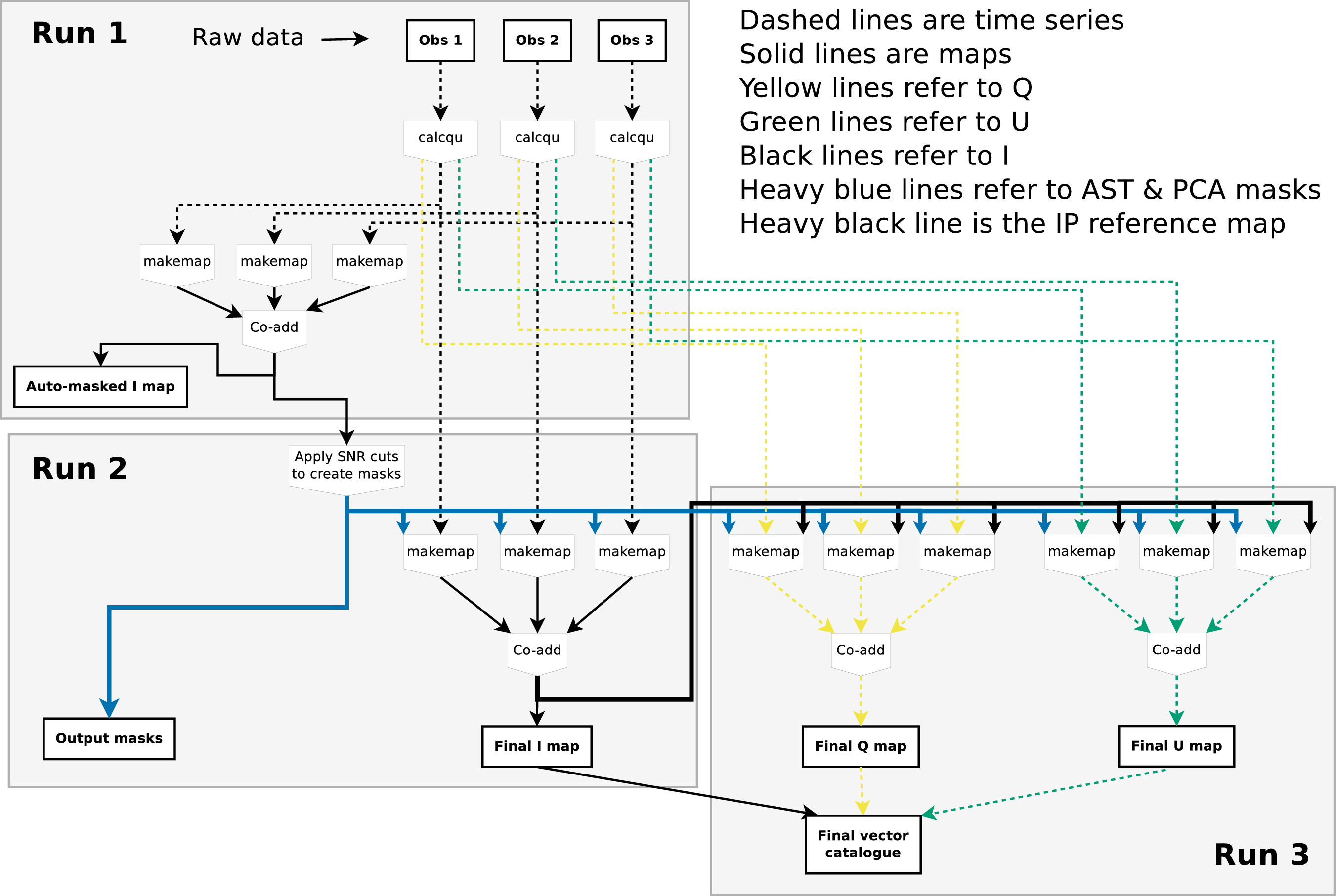
The data reduction process can be broken down into three main stages – referred to as “Run 1”, “Run 2” and
“Run 3” in Figure 3.1.
Step 1
The initial step of the process (see Run 1 in Figure 3.1) creates a preliminary co-added total intensity
() map
from the raw data files for all observations provided to the reduction routine (see Chapter 4).
The process
The analysed intensity values in the raw data time-streams are first flat-fielded and converted into
,
, and
time-streams using the calcqu command. These time-streams are stored for future use in the directory qudata,
specified by the QUDIR parameter in the example command below.
The SMURF:makemap command is then used to create a separate map from the I time-stream for each
observation, using SNR-based “auto-masking” to define the background regions that are to be set to
zero at the end of each iteration. This step uses a PCA threshold of 50 (see Section 3.5 for more
details).
pca.pcathresh = -50
These maps are stored for future use in the directory maps, specified by the MAPDIR parameter. Each map has a
name of the form:
<UTDATE><OBSNUM><CHUNKNUM>imap.sdf
where <CHUNKNUM>
indicates the raw data file at the start of the contiguous chunk of data used to create the map, and is usually
0003.
A co-add is then formed by adding all these maps together. Each individual map is then compared with the
co-add, in order to determine a pointing correction to be applied to the observation in future. These corrections
are stored in the FITS header of the individual maps.
Step 2
In the second step of the process (see Run 2 in Figure 3.1) an improved
map is
produced. These improvements come from
-
(1)
- applying the pointing corrections determined in Step 1,
-
(2)
- the use of an increased number of PCA components (
pca.pcathresh=-150), and
-
(3)
- using a single, fixed mask for all observations. The mask is determined from the preliminary
co-added
map and thus includes fainter structure than would be used if the mask was based on only one
observation.
Step 3
In the third step of the reduction process (see Run 3 in Figure 3.1), both the
and
maps are produced.
The production of the
and maps
requires the and
time-series data (produced
in Step 1), the final
map (produced in Step 2), and the output masks (also produced in Step 2). Once the
and
maps
are produced a final vector catalogue is created.
3.2 MAKEMAP
The POL-2 data reduction builds upon the existing SCUBA-2 Dynamic Iterative Map-Maker, hereafter just
referred to as the “map-maker". This is the tool used to produce SCUBA-2 maps, and is invoked by the
Smurf makemap command. It performs some pre-processing steps to clean the data, solves for multiple signal
components using an iterative algorithm, and bins the resulting time-series data to produce a final science
map.
In pol2map, the map-maker is used in conjunction with calcqu (see Section 3.4) to produce maps of
and
, as well
as .
3.3 SKYLOOP
An option exists to use the Smurf skyloop command to generate maps in place of the Smurf makemap command.
Each invocation of the makemap command creates a single map from the time-series data for a single
observation. If multiple observations are processed together, multiple invocations of makemap are used and the
resulting maps are co-added before moving on to the next step, as indicated in Figure 3.1. The skyloop
command, on the other hand, will process multiple observations in a single invocation, creating a combined
map from all observations. Thus, when using skyloop, Figure 3.1 would be effectively changed such that
each occurrence of “three invocations of makemap feeding one co-add" would be replaced by a
single invocation of “skyloop". See Section 3.7 for more information about the effects of using
skyloop.
3.4 CALCQU
In addition to the POL-2 data reduction building on the existing SCUBA-2 map-maker, pol2map also relies on
the Smurf command calcqu.
This calcqu tool creates time series holding ,
, and
values from a set of POL-2 time series holding raw data values. The supplied time-series
data files are first flat-fielded, cleaned and concatenated, before being used to create the
,
, and
values.
The ,
, and
time-series are down-sampled
to 2Hz (i.e. they contain two ,
, or
samples
per second), and are chosen to minimise the sum of the squared residuals between the measured raw data
values and the expected values given by Equation 2.9.
3.5 PCA
One difference between the reduction of SCUBA-2 data and POL-2 data is the method used to
remove the sky background. The sky background is usually very large compared with the
astronomical signal, and both are subject to the same form of instrumental polarisation (IP—see
Section 2.2). This IP acting on the high sky background values causes high background values in the
and
maps. However,
there is evidence that the IP is not constant across the focal plane, resulting in spatial variations in the background of
the and
maps.
For non-POL-2 data, the background is removed using a simple common-mode model, in which the mean of the
bolometer values is found at each time slice and is then removed from the individual bolometer values. This
ignores any spatial variations in the background, and so fails to remove the background properly in POL-2
and
maps.
To fix this, a second stage of background removal is used when processing POL-2 data, following the initial common-mode
removal. This second stage is based upon a Principal Component Analysis (PCA) of the 1280 time-streams in each
sub-array (the
and
data are processed separately). The PCA process identifies the strongest time-dependent components that are
present within multiple bolometers. These components are assumed to represent the spatially varying
background signal and are removed, leaving just the astronomical signal. You may specify the
number of components to remove, via a makemap configuration parameter called pca.pcathresh
although pol2map, the reduction command for POL-2 data, provides suitable defaults for this
parameter.
- first stage uses
pca.pcathresh = -50
- second stage uses
pca.pcathresh = -150
On each makemap iteration, the PCA process removes the background (thus reducing the noise in the map) but
also removes some of the astronomical signal. The amount of astronomical signal removed will be greater for
larger values of pca.pcathresh. However, this astronomical signal is still present in the original time-series
data, and so can be recovered if sufficient makemap iterations are performed. In other words, the use of larger
values of pca.pcathresh slows down the rate at which astronomical signal is transferred from the time-series
data to the map, thus increasing the number of iterations required to recover the full astronomical signal in the
map.
Spatial variations in the sky background may also be present in non-POL-2 data, but at a lower
level. For a discussion of why PCA is not routinely run on non-polarimetric SCUBA-2 data, see
Appendix A.
3.6 Masking
A mask is a two-dimensional array that has the same shape and size as the final map, and that is used to
indicate where the source is expected to fall within the map. ‘Bad’ pixel values within a mask indicate
background pixels, and ‘good’ pixel values indicate source pixels. Masks are used for two main
purposes:
-
(1)
- They prevent the growth of gradients and other artificial large scale structures within the map.
For this purpose, the astronomical signal at all background pixels defined by the mask is forced to
zero at the end of each iteration within makemap (except for the final iteration).
-
(2)
- They prevent bright sources polluting the evaluation of the various noise models (PCA, COM,
FLT) used within makemap. Source pixels are excluded from the calculation of these models.
The pol2map script uses different masks for these two purposes—the “AST” mask and the “PCA” mask. The
PCA mask is, in general, less extensive than the AST mask, with the source areas being restricted to the brighter
inner regions. Each of these two masks can either be generated automatically within pol2map, or be specified by
a fixed external NDF.
3.7 Tailoring a reduction
Variances between POL-2 maps
MAPVAR is a pol2map parameter that controls how the variances in the co-added
,
, and
maps
are formed.
If MAPVAR is set TRUE, the variances in the co-added
,
, and
maps
are formed from the spread of pixel data values between the individual observation maps. If MAPVAR is FALSE
(the default), the variances in the co-added maps are formed by propagating the pixel variance
values created by makemap from the individual observation maps (these are based on the spread of
,
, or
values
that fall within each pixel).
Use MAPVAR=TRUE only if enough observations are available to make the variances between them
meaningful. A general lower limit on its value is difficult to define, but a minimum of 10 observations is
advised.
If a test of the effect of this option is required on a field for which the
,
, and
maps
from a set of individual observations are already available, the following may be done:
% pol2map in=maps/\* iout=imapvar qout=qmapvar uout=umapvar mapvar=yes \
ipcor=no cat=cat_mapvar debias=yes
assuming that the ,
, and
maps are in directory maps. The variances in imapvar.sdf, qmapvar.sdf and umapvar.sdf will be
calculated using the new method, and these variances will then be used to form the errors in the
catmapvar.FIT
catalogue.
In general, within the source regions, the variances created using MAPVAR=TRUE will be larger than those created
using using MAPVAR=FALSE (within background regions there should be little difference). This is partly caused
by residual uncorrected pointing errors, which have a particularly large effect near bright point sources if
MAPVAR=TRUE.
It is also partly caused by intrinisic instabilities within the iterative map-making algorithm, which allow
low-level artificial extended structures to develop within the source regions defined by the AST mask. Such
artificial structures will vary from observation to observation, and so will contribute to the variances calculated
using MAPVAR=TRUE.
Two options are provided by pol2map that may be useful in reducing the larger-than-expected dispersion
between maps made from different observations.
-
(1)
- Setting the parameter
OBSWEIGHT=TRUE when running pol2map will cause each observation to be
assigned a separate weight, which will be used when forming the co-add of all observations. This
will affect both the data values and the variances in the resulting co-add. The purpose of these
weights is to down-weight observations that produce maps that are very dissimilar to maps made
from the other observations.
Without this parameter setting, the co-add is formed using weights equal to the reciprocal of
the pixel variance values in each individual observation’s map. As mentioned above, these pixel
variance values can sometimes seriously underestimate the dispersion between observations. For
instance, observations that are clearly bad (e.g. out of focus) can have relatively low pixel variance
values, and thus be included with high weights in the final co-add.
If the OBSWEIGHT parameter is set TRUE, each observation is given an additional weight that is used
to factor the per-pixel weights derived from the pixel variance values, in order to down-weight
observations that are clearly bad. To form these weights, an initial co-add is formed using equal
weights for all observations. The maps made from the individual observations are then compared
with this initial co-add, and each observation is assigned a weight equal to the reciprocal of the
mean squared residual between the individual observation’s map and the initial co-add (any
required pointing correction is applied to the individual observation map before forming these
residuals). The calculation of the mean squared residual is limited to those pixels inside the AST
mask (i.e. source pixels). The weights derived in this manner are normalised to have a median
value of 1.0, and any normalised weights larger than 1.0 are reduced to 1.0. An improved co-add
is then formed using these observation weights.
Another iteration is then performed, in which individual maps are compared with this improved
co-add and new weights are derived. This iterative process continues until the typical error in the
middle of the co-add stops falling significantly.
-
(2)
- Setting the parameter
SKYLOOP=TRUE when running pol2map will cause maps to be made using
the SMURF:skyloop command, instead of makemap. In the context of the skyloop documentation,
one “chunk” of data usually corresponds to a single observation.
A single invocation of skyloop creates an ,
,
or
map from all supplied observations, using a method that attempts to minimise the intrinsic instabilities
of the map-making algorithm within the AST mask. It should be noted that convergence can
require a significantly greater number of iterations when using skyloop than when using makemap.
Also, skyloop requires much more disk space than makemap.
The skyloop command combines all observations together at each iteration of the map-making
algorithm. Since the spurious large-scale structures created at each iteration are independent of
each other, taking the mean of the maps after each iteration reduces the level of such structures,
and prevents them from growing in amplitude on successive iterations due to the instability in the
map-making algorithm.
The above two methods can be used together by supplying TRUE values for both OBSWEIGHT and
SKYLOOP.
Note, it is not recommended to use MAPVAR=TRUE or SKYLOOP=TRUE on Step 1 (i.e. when creating the auto-masked maps).
Doing so is of no benefit to the final maps and can cause problems such as negative bowling.
If the OBSWEIGHT parameter is used at Steps 2 or 3, then it must also be used at Step 1.
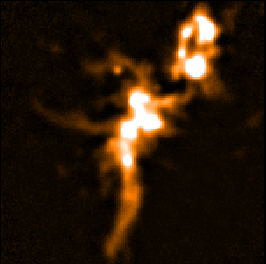
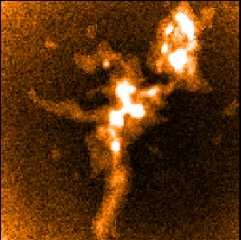
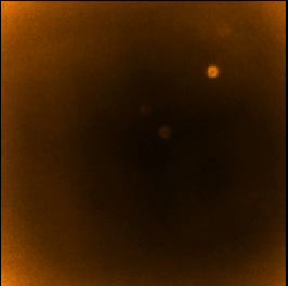
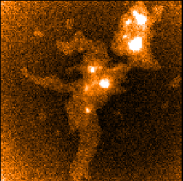
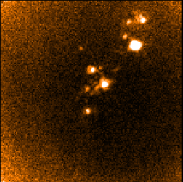
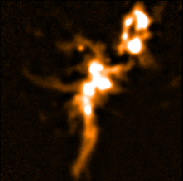
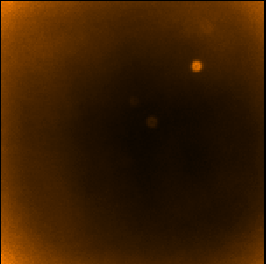
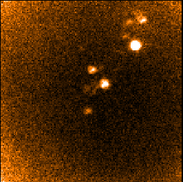
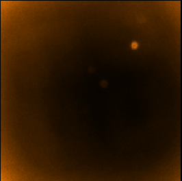
The following panels show the effects of using SKYLOOP and OBSWEIGHT on a total-intensity mosaic of 21
observations. All data-value maps are shown with a single scaling, and all standard-deviation maps are shown
with a single scaling (different from the scaling for the data-value maps).
For comparison, below are the equivalent auto-masked maps made by Step 1.
Copyright © 2021 East Asian Observatory