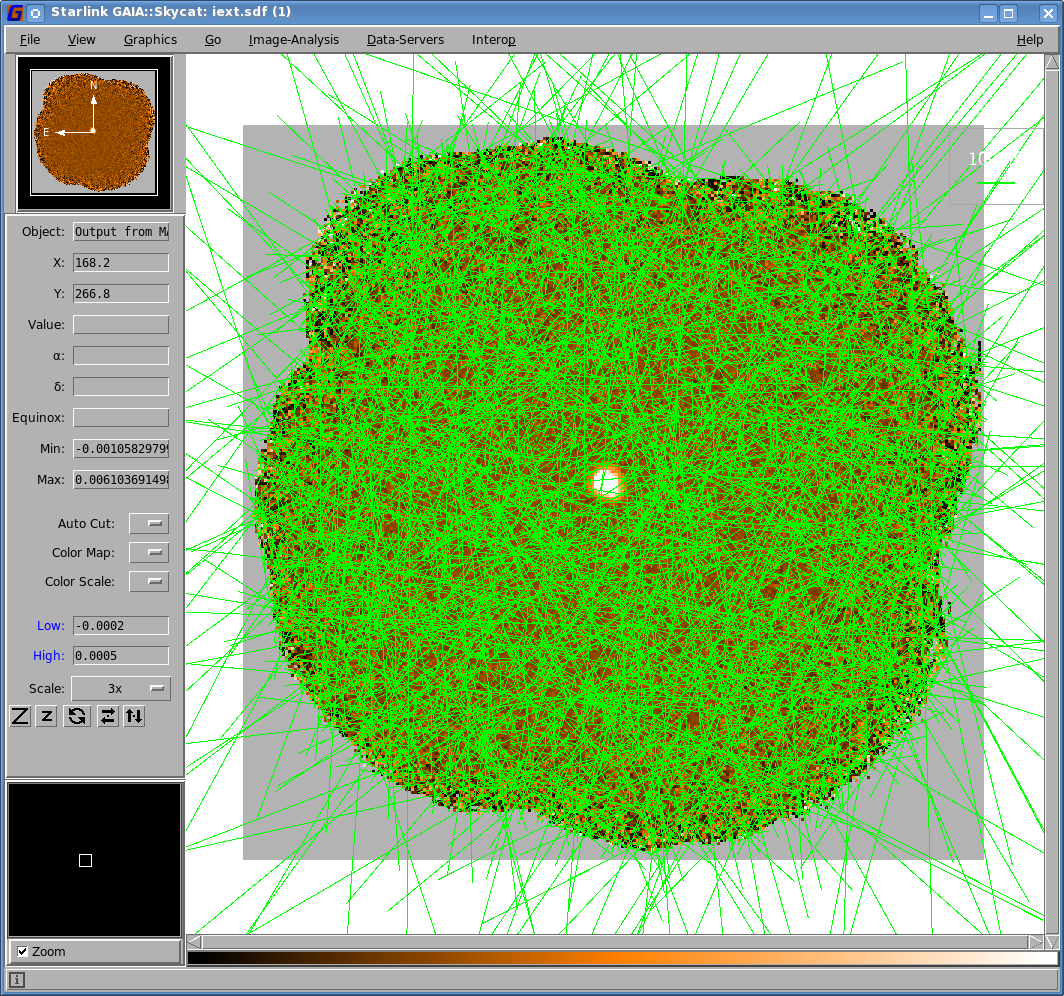
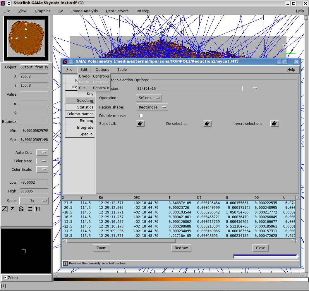
Figure 5.1: Left: Opening up the polarimetry toolbox in Gaia. Right: The initial POL-2 vectors
overplotted in Gaia.
The Starlink package Gaia can be used to inspect the results of the data reduction. To plot the output vector catalogue onto the final total intensity map, first open up the map in Gaia.
From the main Gaia window, select the drop-down menu option Image Analysis / Polarimetry toolbox. This
should launch a new toolbox window entitled GAIA: Polarimetry. From this window, use the drop-down menu
option File / Open to load the file mycat.FIT. This should then populate the lower part of the window with the
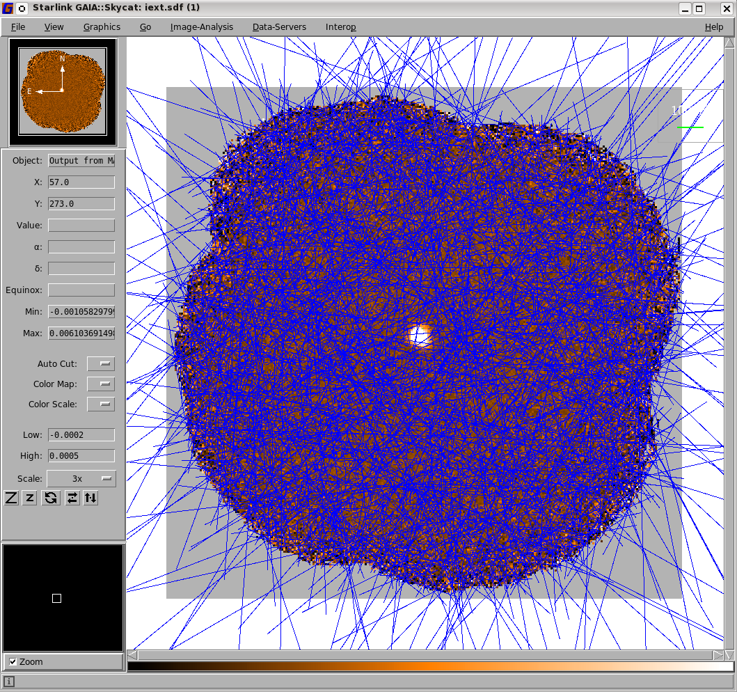
contents of this polarimetry catalogue file. Each of the vectors in this file will be automatically overlaid on the
main image window (see Figure 5.1).
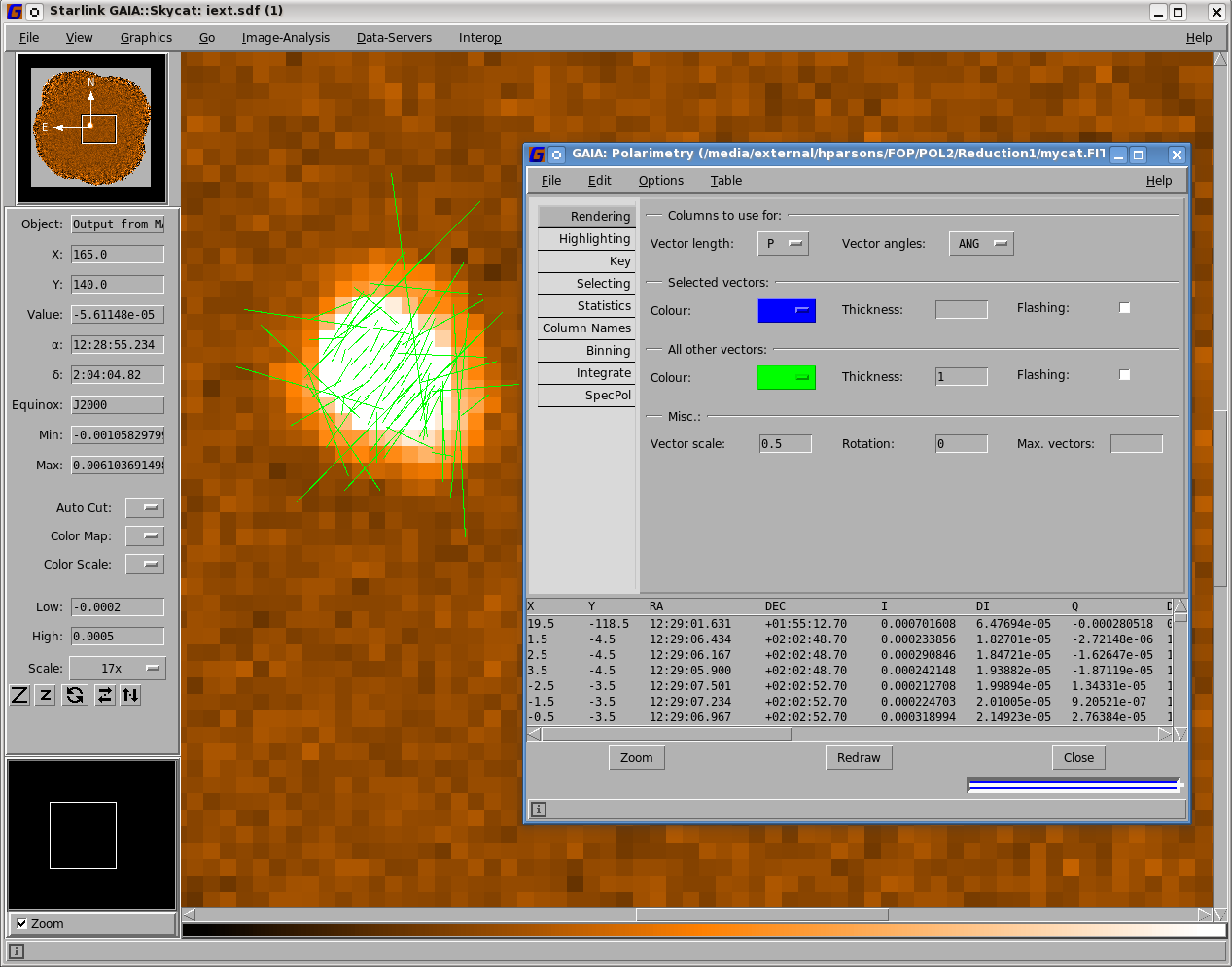
In order to filter the number of overlaid vectors down to a more useful number and size, the various options in the GAIA: Polarimetry toolbox can be used. First, select the Rendering tab on the left hand side. This will reveal a panel that will indicate which quantities are currently being used for the vector overlays. In this case, the vector length is taken from the P column of the table, and the vector angles are taken from the ANG column.
Currently the figure has too many vectors to be scientifically meaningful. To filter out most of the extraneous vectors, click on the Selecting tab, and set the Expression field to be the following:
Ensure that “Return” is pressed after entering the above expression.
The above expression selects the data points in the polarimetry table that have an associated total intensity (Column I) less than 10 times the associated error value for that intensity (Column DI). To remove all of these extraneous vectors, either press control-X or use the drop-down menu option Edit / Cut. This should leave just a small number of vectors clustering around the target object (see Figure 5.2) 1.
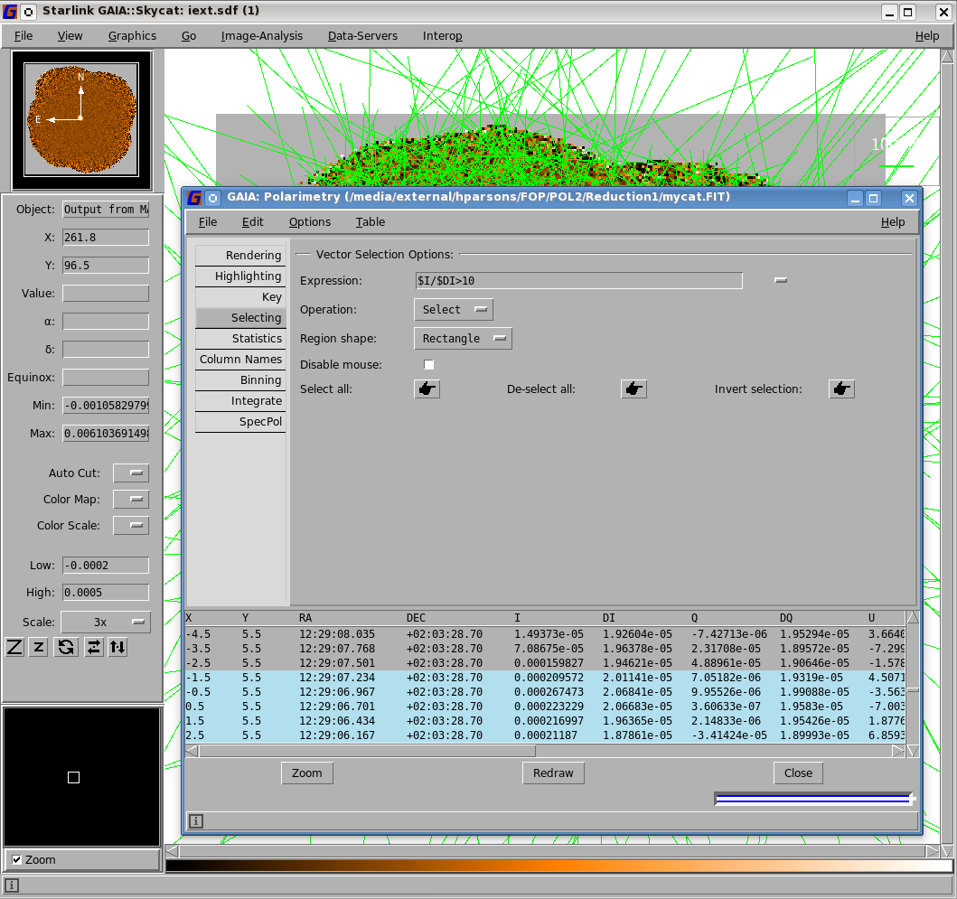
$I/$DI10.
This will only plot vectors with an intensity signal-to-noise ratio greater than 10 in Gaia. To ensure that
this is specified, ensure that “Return” is pressed after entering the expression. Right: After selection, the
selected vectors are shown in blue. Zooming in on the central region of the map makes it possible to view the vectors near the target object (see
Figure 5.3). If needed, it is possible to change the vector scale by selecting the Rendering tab in the "GAIA:
Polarimetry" window.
Finally it is useful for future use (as in the examples in the following sections) to save the final selection of vectors. To save the displayed vectors to a new catalogue, use the drop-down menu File / Save in the polarimetry toolbox.
It is possible to use Kappa and Polpack to create POL-2 plots.
Note that in the following examples, it will be necessary to ensure that only the vectors to be plotted are
included in the file mycat.FIT.
There are two main ways to do this — either by saving the output catalogue from Gaia or using the Starlink package Polpack to manipulate the catalogue produced by the user. To use Polpack, simply run:
then select the vectors of interest.
The use of the Polpack polselect command is generally recommended over the use of the Cursa catselect command when working with POL-2 datasets, as it provides a greater number of options specifically designed for use with POL-2 data. For example, polselect offers additional modes that allow the specific selection of vectors that are located within a given region on the sky (specified by an ARD or AST region description), or which correspond to pixels with good values in a specified mask NDF.
For more info, see http://pipelinesandarchives.blogspot.com/2015/02/better-fonts-in-postscript-output-from.html
Graphics-related attributes that can be set are described in SUN95: Descriptions of Plotting Attributes, and the coordinate system attributes that can be set are described in SUN/95: Descriptions of Frame Attributes.
In this example, an output file, plot1.pdf, is created from the input catalogue mycat.FIT.
Select a higher quality PostScript font (Times New Roman in this case):
Select the PostScript graphics device, writing to file plot1.ps:
For convenience, create a text file holding the main plotting style for polplot:
Likewise, create a text file holding the style for the vector length key:
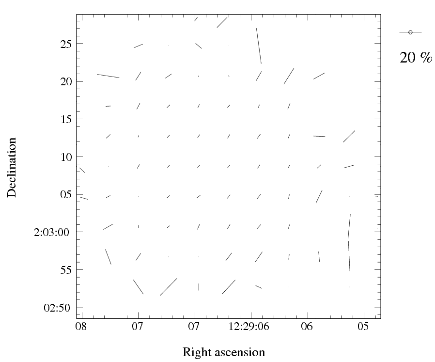
Plot the vector map. The vscale parameter controls the vector scale, and the keyvec parameter controls the
length of the vector used as the key. There are many other parameters that can be used to control the behaviour
of polplot—see the Polpack manual (SUN/223):
Convert the map into a PDF file and remove blank margins (if required):
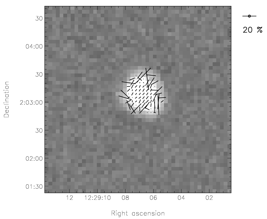
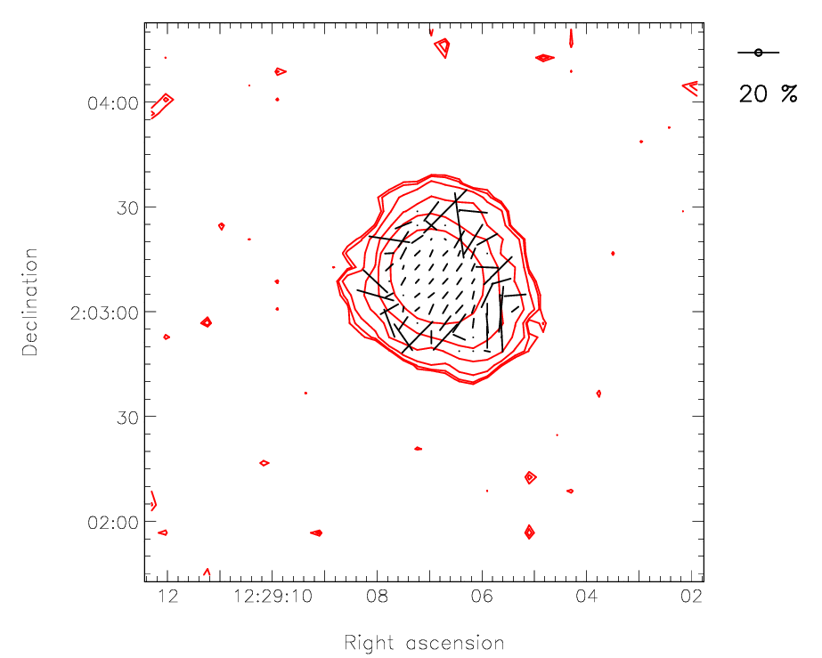
In this example, an output file, plot2.pdf, is created from the input catalogue mycat.FIT.
Select the PostScript graphics device, writing to file plot2.ps. Note that in this example, a value is
not assigned to the PLOT_PS_FONT environment variable. This means that the resulting plot uses
the default PGPLOT fonts, rather than the higher quality PostScript fonts used in the previous
example:
Set up the main plotting style for contour and polplot:
Produce the contour map as follows:
Modify the above style for the vector map to produce black vectors:
Set the style for the vector length key:
Plot the vector map over the contour map. The vectors and contours are aligned automatically in sky coordinates:
Convert into a PDF file and remove blank margins (if required):
In this example, an output file, plot3.pdf, is created from the input catalogue mycat.FIT. First,
select the appropriate PostScript device (the default PGPLOT fonts are use again, as in the previous
example):
To ensure a monochrome colour table is used for the image run lutgrey:
Set the main plotting style for display and polplot:
The following function is used to reduce the dynamic range in the map. This allows the user to be able to see structure in the fainter parts, without saturating the brightest regions):
Display the image, using a reduced range of colours (pens) so that the darkest regions are grey rather than black. This means the black vectors can still be seen within the dark regions:
Modify the above style for the vector map to produce wider vectors:
Set the style for the vector length key:
Plot the vector map over the contour map. The vectors are aligned automatically with the map:
Convert into a PDF file and remove blank margins (if required):
Catalogues produced by pol2map can be explored using the popular Topcat catalogue browser (see http://www.starlink.ac.uk/topcat/). For instance:
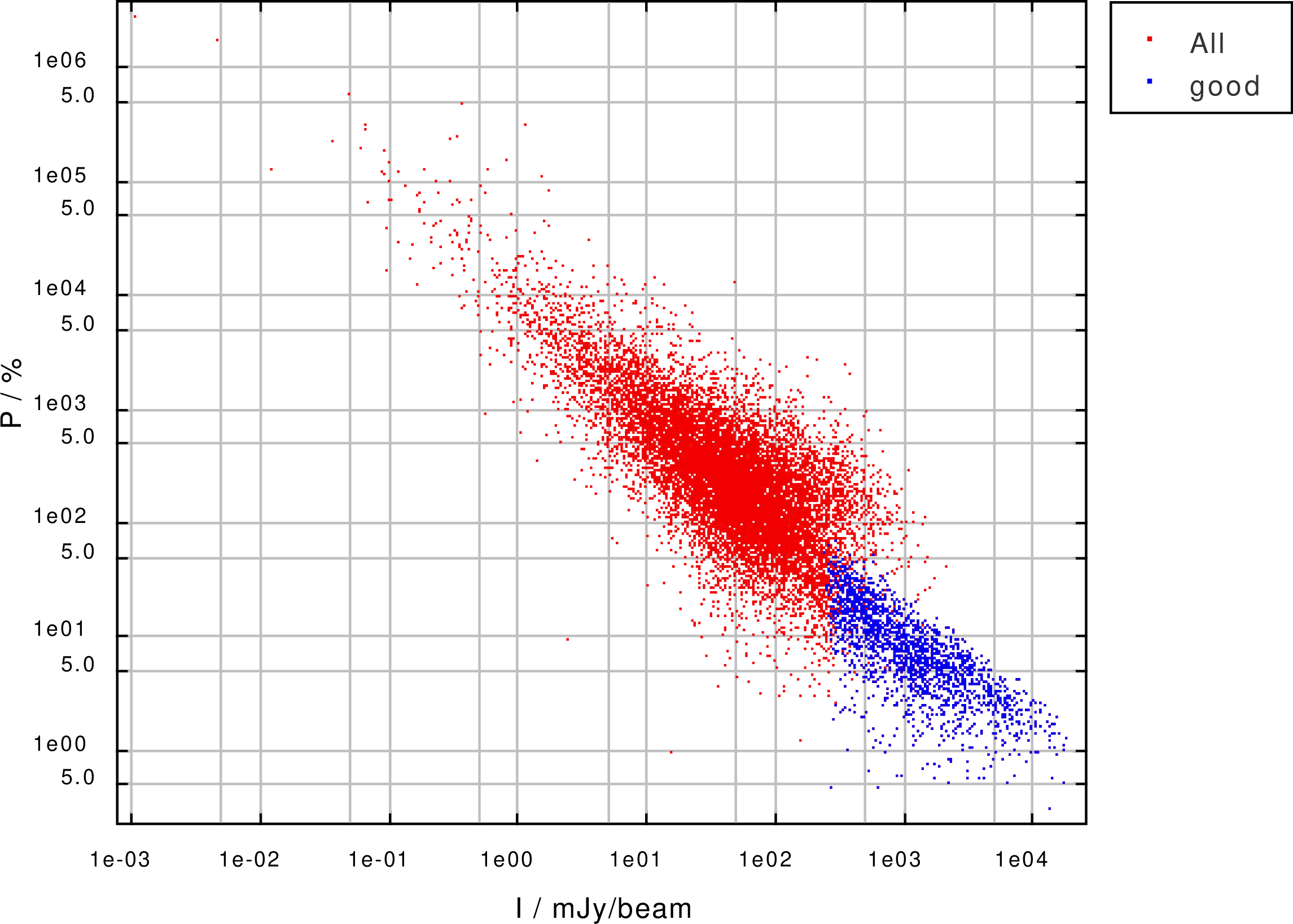
Unlike the other tools described above, Topcat cannot produce a visualisation of the catalogue as a set of vectors. However, it goes well beyond the facilities of the other tools in allowing the user to explore correlations between different quantities in the catalogue via two- and three-dimensional scatter plots—see Figure 5.7. It can also be used to cross-correlate two different catalogues, create subsets of a catalogue, create new columns containing related quantities, etc. It also allows the modified catalogue to be saved to a new catalogue file on disk. However, users should be aware that any such new catalogue will not contain the WCS information required by other Starlink applications to perform WCS-related operations, such as displaying annotated axes and aligning data-sets. This WCS information can be copied back into the new catalogue, however, using the polwcscopy command (Section 6.4).
1This example is provided here for simplicity. It should be noted, however, that a selection criterion following the general format of
$I/$DI<10 || $AST==0 might actually further improve some selections, as it makes use of the AST column to remove vectors outside the AST
mask (i.e. background vectors).