|
||||||||||||||
 |
||||||||||||||
|
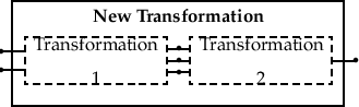
Figure 1: Concatenating two transformations.
As well as providing routines for applying compiled mappings to 1- and 2-dimensional data (Sections 3.6 & 3.7), the TRANSFORM facility also has a set of routines for applying more general mappings. These are appropriate, for instance, when the number of input or output data coordinates is greater than 2 (or when these numbers are unequal) or when the number of coordinates is not known in advance. In such cases, all the input and output coordinates must each reside in single data arrays.
These general routines have names of the form TRN_TRNx, where x is either I, R or D according to whether the data are specified by integer, real or double precision values respectively. Thus, to transform a general set of data points specified by an array of real coordinates, the routine TRN_TRNR would be used, thus:
where:
In the following, a set of data points representing a 3-dimensional object is converted into a related set of 2-dimensional points using TRN_TRNR. The resulting points are then plotted using GKS. With a suitable choice of mapping, such an arrangement might be used to generate perspective pictures of 3-dimensional objects:
Programming notes:
During the process of transforming coordinate data, numerical errors (such as division by zero or overflow) will inevitably occur from time to time. There is no need to include specific protection against this when a transformation is formulated, however, because such errors will automatically be trapped and converted into one of the standard Starlink bad values.4
This form of error trapping is performed by all the routines which apply compiled mappings to coordinate data. The resulting “bad coordinates” will, where necessary, be propagated through each stage in the evaluation of a compiled mapping, so that all the results which have been affected by numerical errors can later be identified. No error report is currently made (or STATUS value set) if a numerical error of this nature occurs.
All the routines which apply compiled mappings to coordinate data can also recognise bad coordinate values supplied as input, and will propagate these if required. Frequently, however, there will not be any bad coordinates in the input data stream and it may be possible to save appreciable amounts of processing time by disabling recognition of these values (thereby eliminating unnecessary checking), especially when large arrays are being processed. Each relevant routine therefore carries a logical argument called BAD, which specifies whether recognition of bad input data is required (execution will generally be faster if BAD is .FALSE.). Note that this argument only affects recognition of bad data in the input stream, while numerical errors which occur during the computation are always converted into bad values and correctly propagated to the output.
It is common to find that the relationship between two coordinate systems is most easily expressed in terms of several transformations applied in succession. For instance, the transformation between positions on the sky and the pixel coordinates of a CCD image might be divided into two stages; the first representing the effect of imaging the sky into the focal plane of the telescope, and the second taking account of the position, size and orientation of the detector in the focal plane. The TRANSFORM facility makes explicit provision for cases such as this by allowing transformations to be concatenated.
A rather general case of concatenation is illustrated in Figure 1. In this example, Transformation 1 relates two input variables to three “intermediate” variables , which are also the input variables of Transformation 2. This transformation, in turn, has a single final output variable . The concatenation process involves eliminating the three intermediate variables and storing the two transformation definitions together in a single new transformation. This new transformation then has two input variables and a single output variable . Using the ‘.’ symbol to represent concatenation, this entire process may be summarised as:
or, in general:
Note that the number of output variables from the first transformation must be equal to the number of input variables to the second transformation. For obvious reasons, also, it is not permitted to concatenate a transformation in which only the forward mapping is defined with another in which only the inverse mapping is defined (e.g. [] could not be concatenated with []).
The result of concatenating two transformations is itself a transformation, so the process may be repeated indefinitely, making it possible for a whole sequence of transformations to be joined together and processed as a single unit. Once transformations have been combined in this way, however, they cannot later be separated.
Concatenation of a pair of transformations is performed by the routine TRN_JOIN (concatenate transformations), as follows:
where:
As with the TRN_NEW routine (Section 3.3), a temporary transformation may also be produced by leaving the ELOC argument (and optionally the NAME argument) blank when TRN_JOIN is invoked.
In addition to producing new transformations by concatenating existing ones, it is also possible to modify an existing transformation by prefixing or appending another one to it. For example, to prefix one transformation to another, TRN_PRFX (prefix transformation) would be used, thus:
In this case, the two transformations with locators LOCTR1 and LOCTR2 are concatenated (as above), but the resultant transformation replaces the second one, so that the first transformation is, in effect, prefixed to it. The first transformation itself is not altered.
The routine TRN_APND (append transformation) behaves in a similar way, except that it appends the second transformation to the first. In this case the second transformation remains unchanged.
Suppose LOCTRS is a locator to a transformation which relates the pixel coordinates of a CCD image to positions on the sky . If the size of this image is altered during data reduction, then its pixel coordinates will change and the astrometric calibration will need adjustment to take account of this.
If the and pixel coordinates are reduced by (say) 19 and 25 units, then a transformation inter-relating the old and new pixel coordinates could be formulated as follows:
| (4) |
and then created. This transformation (with locator LOCTRA, say) represents the necessary adjustment which should be applied as a prefix to the original transformation, thus:
The modified transformation (LOCTRS) will then correctly relate the image’s new pixel coordinates to positions on the sky, the necessary adjustment having been achieved through the following concatenation process:
Note that it is not necessary to know anything about the nature of the original transformation [] in order to apply such a correction.
Inversion of a transformation is a straightforward process involving the inter-change of the forward and inverse mappings (the numbers of input and output variables will also be inter-changed). It is performed by TRN_INV (invert transformation), thus:
where LOCTR is a locator to the transformation to be inverted. After such a call, compiling the transformation in the forward direction will yield the same compiled mapping as would have been obtained by compiling in the inverse direction prior to calling TRN_INV.
The main use for TRN_INV is in adapting transformations which have been created or supplied the “wrong way round” for some purpose (e.g. concatenation with another transformation).
To simplify the process of formatting transformation functions, a set of routines is provided which allows numerical or textual values to be inserted into “template” character strings. These routines largely eliminate the need to use Fortran WRITE statements to construct transformation functions containing numerical values.
The routines have names of the form TRN_STOK[x], where x is either I, R or D according to whether the type of value to be inserted is integer, real or double precision respectively. The routine TRN_STOK (i.e. with x omitted altogether) is used for making textual (rather than numerical) insertions but otherwise functions in the same way. These routines rely on the concept of a token,5 which is placed in a character string at the point where an insertion is to be made and which is subsequently replaced by the value to be inserted. For example, if the character variable TEXT had the value:
then TRN_STOKR (substitute a real token value) could be used to substitute a numerical value for the ‘zero_point’ token, as follows:
This causes all occurrences of the ‘zero_point’ token to be replaced with the formatted real number ‘17.7’, while NSUBS returns the number of substitutions made (in this case there will only be one). The value of TEXT then becomes:
Note that the TRN_STOKx routines will respect the syntax of transformation functions, so that negative numerical values will be enclosed in parentheses before a substitution is made. For instance, if the call to TRN_STOKR had been:
then the ‘zero_point’ token would be replaced by ‘(-17.7)’ to prevent the illegal expression
‘…+ -17.7’ from being produced. The need for two extra characters to accommodate these parentheses
must be remembered when declaring the size of character strings.
This illustrates the use of TRN_STOKR in a subroutine to “package up” the creation of a simple [] transformation which contains several adjustable numerical parameters. The same principles can be followed to write routines for creating a variety of specialised transformations.
Programming notes:
This simple example formulates a set of transformation functions to multiply each ordinate of a 3-dimensional coordinate system by 2.0 to yield the coordinates :
The following constructs an expression representing a polynomial in with an arbitrary number of numerical coefficients:
Programming notes:
The effect of this algorithm with (say) the 5 polynomial coefficients 0.1, 0.12, 1.06, 4.4 & 1E7, would be to produce the following expression:
which casts the polynomial into a form for efficient evaluation using Horner’s method.
4The Starlink bad values are symbolic constants with names of the form VAL__BADx, where x is either D, R, I, W, UW, B or UB according to the data type in question. These constants are defined in the include file PRM_PAR (see SGP/38 & SUN/39 for further information).
5Tokens take the same form as the variable names used in transformation functions – i.e. they may contain only alpha-numeric characters (including underscore) and must begin with an alphabetic character. Tokens may be of any length and may use mixed case (token substitution is not case-sensitive) but embedded blanks are not allowed.