Appendix I
Removal of reference signal

During heterodyne observations, the telescope switches (see Section 3.3.2) between observing your target and a nearby reference position. The latter’s spectrum is subtracted from the target data in order to subtract the sky-background signal.

In most cases, this reference location will be devoid of source emission. However, around the Galactic Plane and especially the Galactic Centre, it can be problematic to find a reference position that’s pointing at sky, even with a position switch. Should the reference measurement include a source, its signal will be subtracted from all the spectra in your data, appearing one or more absorption lines. If the absorption occurs where your target has strong emission across a wide range of frequencies, the absorption feature can easily be camouflaged. Even it is located where there is weak or no target signal, a strong absorption feature will slightly bias the baseline fitting. So if your data has such artefacts, it is worth trying to correct them.

A simple approach for removal is to interpolate across the absorption feature, but this does assume that the target emission is not varying across the width of the absorption line or lines. If the absorption is located clear of your source’s emission, it is possible to merely mask the feature with chpix. The following example masks all spectra witihn the time-series cube ts_cube between 3.5 and 7.8 km s$-1$.

Figure I.1: This shows a spectral cube collapsed to two dimensions with the "Collapse" tag, on which a polygonal region of background is outlined. First select the median "Combination method" and then the polygon "Define region" button (both ringed). Click the left mouse button to add points, and double-click to complete the polygon. Vertices may be dragged or new vertices added. See the Gaia help for details.

Figure I.2: This shows a median spectrum from a Gaia region defined as in Figure I.1. Use the marked "File" menu and choose "Save as NDF" to save the created spectrum.

The basis of a better method is to attempt to determine the reference spectrum. One such approach is to identify regions with none or minimal target emission in your reduced spectral cube, mask these, then form the median spectrum of the remainder. Regions to include or exclude may be defined with ARD regions in a text file, possibly created with Gaia(see Section 8.7); or using the shape selection in the Gaia cube-manipulation controls, especially the polygon (see Figure I.1). 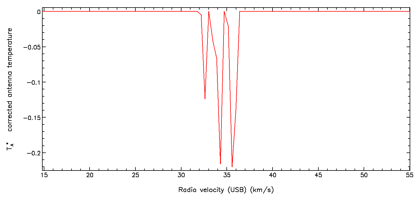The resultant spectrum may be saved (see Figure I.2). In practice this median spectrum will likely still have some target emission and possibly a non-flat baseline, which need to be removed. One approach is to smooth the spectrum with a wide kernel—essentially a low-pass filter—and then subtract the smoothed spectrum from the original. Finally, since we are only interested in the aborption features, set all the non-line elements to 0. In the Figure I.2 example that is between 4.7 and 6.3 km s$-1$.

Figure I.3: An extract from an estimated spectrum derived from the methods outlined in the test. Note that beyond the lines, pixel values are zero so as not to add noise to the cube once the reference spectrum is subtracted.

To apply this to your cube, enlarge it to the dimensions of your cube. The value of the AXES parameter will depend on whether you intend to subtract the reference spectrum from the raw time series, or from the position-position-velocity (PPV) reduced cube. For the time series

and for the PPV

AXES specifies the axis to retain (1) or new dimensions to grow (0). The pixel bounds of the new axes are given repectively by LBOUND and UBOUND arrays. In the time-series example, there are 14 receptors and 4202 spectra. You can find the bounds of your cube with ndftrace.

I.1 Remove the reference signal using ORAC-DR

A number of recipe parameters are provided for the attempted removal of reference signal, and are listed in Table G.12. For Galactic Plann surveys the following combination have worked moderately well.

You may need to enlarge REF_EMISSION_BOXSIZ should your data have narrow velocity channels. An example of using these settings that successfully removed the reference signal from some Galactic Plane data is shown in Figure I.4.

Figure I.4: Part of a mean spectrum collapsed over a COHRS[13] tile in the Galactic Plane. The red curve shows the original uncorrected spectrum and the blue curve is the re-processed spectrum, where the absorption feature is removed within Orac-dr using the primary set of recipe parameters listed in the text above.

The algorithm used by Orac-dr does not always remove all of the lines, and in rare cases leaves lines unchanged. For these recalcitrant lines some additional facilities are provided, where you set the velocity limits of the reference absorption line.

REF_SPECTRUM_REGIONS sets a comma-separated list of the velocity ranges of the absorption lines.

If that does not work, you can provide your own estimated reference spectrum, containing zeroed data values outside of the line extent, as described earlier and shown in Figure I.3. You then supply its file name using the recipe parameter shown below.

The algorithms used are described in a forthcoming COHRS [13] Second Release paper.