Processing math: 100%
Chapter 3
The Dynamic Iterative Map-Maker Explained
The Dynamic Iterative Map-Maker, hereafter just referred to as the map-maker is the tool you will use to
produce SCUBA-2 maps, and is implemented by the Smurf makemap command. It performs all pre-processing
steps to clean the data, followed by solving for multiple signal components using an iterative algorithm, and
binning the resulting time-series data to produce a final science map.
The makemap command can be invoked in two ways: 1) directly by typing “makemap” in response to a unix
shell prompt (see Section 5), or 2) indirectly as part of an Orac-dr recipe (see Chapter 4).
This chapter describes how the map-maker produces a science image from raw SCUBA-2 data. It should be
considered essential reading as it provides an understanding of how your reduced image was produced.
This is particularly true if you wish to modify the default map-maker parameters. If you prefer to jump
straight in to the data reduction go to Chapter 4.
3.1 How it works
The time-varying signal recorded by a bolometer, b(t),
contains contributions from a variety of sources:
|
b(t)=e(t)×a(t)+nw(t)+gnc(t)+nf(t), | (3.1) |
where e(t) is the
atmospheric extinction, a(t)
is the astronomical signal (time varying as the telescope scans across the sky),
nw(t) is the uncorrelated
white noise, g
is an optional scalefactor which is unique to each bolometer,
nc(t) is the correlated (or,
common mode) signal, and nf(t)
is the (predominantly low-frequency) noise which does not have a simple correlation relationship that would be
included in the nc(t)
noise term.
The map-maker works by producing individual models of the various components that make up the signal
recorded by each bolometer. It models and removes the extinction and noise components in order of decreasing
magnitude, ultimately leaving just the astronomical signal plus residual noise. The modelled components are
listed in Table 3.1 and described more fully in Section 3.3.
A configuration file should usually be supplied when running makemap directly. This file holds a set of
parameter values that control all aspects of the map-maker, including details of the pre-processing steps,
which model components to include, parameters that control the determination of each model,
and the stopping (or convergence) criteria. If no configuration file is supplied when running
makemap,
a set of default parameter values will be used. There are a great number of these parameters, but fortunately not
all of them are of interest to the typical user. Appendix I documents the parameters you are more likely to find
of interest, including the default value that is assigned to each parameter if you do not give it a value in your
configuration file. For a full list of all available parameters, see the appendix “Configuration Parameters” within
SUN/258.
It is possible to create a map without supplying a configuration file to makemap (i.e. leaving all configuration
parameters set to their default values—“config=def”—when running makemap) but it is not recommeneded
since it will not give optimal results for your particular observation. For this reason, specialised configuration
files have been developed which are tailored to different science goals, be they detecting faint galaxies or
mapping large molecular clouds. A description of these specialised configuration files can be found in
Section 3.7.
Note: When using the pipeline to create a map, rather than running makemap directly, the pipeline will always
use a configuration file—one of the standard configuration files will be selected if none is specified by
you.
3.2 The reduction step-by-step
This section describes the basic map-making process used by the default configuration. It may be modified in
many ways by supplying a configuration file containing alternative parameter values.
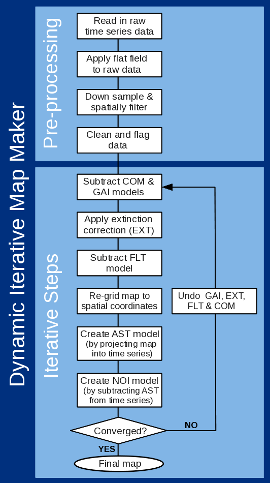
Figure 3.1 shows the flow chart of the basic map-making process. It is divided into two sections: the
pre-processing stage where the data are cleaned, then the iterative stage where the different models are
subtracted, a sky map created and the convergence checked.
-
Initial cleaning and down-sampling
- The separate raw data files are first concatenated into a single
time series for each sub-array (if possible—see Data Chunking) and have the flat-field from the
associated fast-flat scans applied to calibrate the bolometers. This resulting time-series are in units
of pW.
These time-series are then re-sampled at a rate that matches the requested pixel size—the
equivalent to applying a low-pass filter. Down-sampling saves time and memory usage when
running the map-maker, without losing any significant information. The degree of down-sampling
applied depends on how fast the telescope was moving during the observation, the requested
pixel size. In general, slower scans will be more heavily down-sampled than faster scans, and fast
scans may not be down-sampled at all.
A number of cleaning steps are then run: bolometers that have unusually high noise levels
are identified and excluded from further processing, any sudden steps in the base-line of each
bolometer are identified and corrected, and a polynomial estimate of the base-line is removed from
each bolometer.
-
Iterative steps
-
Next comes the iterative stage. In each iteration, estimates are produced for each model
component. These are removed from the cleaned time-series data and the remaining data values
are binned into a map. However, in general, the presence of astronomical signal within the original
time series will have upset the estimates of the COM, GAI and FLT models, causing the final map
to be inaccurate. But now that we have a map (albeit an inaccurate map), we can sample the
map at the position of each bolometer value to get an estimate of the astronomical component
within the original time-series data. We then remove this astronomical signal from the original
time-series data and re-estimate the models. These new model estimates should be more accurate
since they are not so heavily influenced by the astronomical signal. In turn, this allows us to create
a more accurate map. We repeat this process until the map does not change significantly with
further iterations. Whilst not mathematically rigorous, we expect the process to converge because
the astronomical signal is in general much smaller than any of the other components and so each
iteration introduces a very small fractional change in the model estimates.
Within each iteration, the first components to be modelled and removed are COM and GAI, which
work together to calculate and remove the average signal template of all bolometers, allowing each
bolometer to have an arbitrary gain and offset. In addition, the GAI model will flag as unusable
any bolometer in which the signal looks very different to the common-mode.
The next model (EXT) applies a multiplicative extinction correction to the data. Following this,
the FLT model filters each bolometer time-stream independently to remove low frequencies that
correspond to angular scales larger than 600 arcsec and 300 arcsec at 450μm
and 850μm,
respectively.
After these models have been removed, the AST model (i.e. the estimate of the astronomical signal)
produced by the previous iteration, is added back onto the remaining time-series data,
and the new values are binned up on the sky to produce a new estimate of the final science map.
Since many samples typically contribute to the estimate of the signal in a given pixel, the noise
is greatly reduced compared with the time-series data. The variance of each map pixel value is
determined from the spread of sample values that contribute to the pixel. The value of this map
at the position of each bolometer sample is then found. This forms the new AST model which is
removed from the time-streams, leaving just the residual noise.
The NOI model then measures the noise in the residual signals for each bolometer to establish
weights for the data as they are placed into the map in subsequent iterations. This is only done on
the first iteration. Subsequent iterations re-use the weights established on the first iteration.
-
Checking convergence
-
Convergence is checked against the parameters detailed in the configuration file. Convergence
is achieved either when the requested number of iterations has been completed, or when the
mean change in the map pixel values is less than a specified fraction of a standard deviation (see
parameter maptol). If more iterations are required or (in the latter case) the map is still changing
significantly, all the model—except for AST—are added back onto the residuals, thus reconstructing
the original time-series but without the astronomical signal. This is the signal upon which the
model estimates will be based on the next iteration.
For full details of the map-maker see Chapin et al. (2013) [5].
|
|
| Model | Description |
|
|
COM | Common-mode signal |
GAI | Gains that scale each bolometer to the common-mode |
EXT | Extinction correction |
FLT | Filter that removes low frequencies |
AST | Astronomical signal |
NOI | Residual noise |
|
|
| |
Table 3.1: Table adopted from Chapin et al. (2013). A detailed explanation of each model is given in
Section 3.3.
Data Chunking Chunking occurs when there is insufficient computer memory available for the map-maker to
process all the time-series data together, or when there is a gap in the data (e.g. from a missing sub-scan). In
these cases, the map-maker divides up the time-series data into a number of “chunks” and produces a map
from each chunk independently, before re-combining all the maps at a later stage to create the final map.
Ideally you want your data reduced in a single chunk, however this can be unfeasible for large
maps.
The more data the map-maker processes at once, the better chance it has of determining the difference between
sky signal and background noise.
Information about chunking can be obtained in several ways:
- The screen output generated by makemap will include one or more statements about chunking, such
as:
smf_iteratemap: Continuous chunk 1 / 1 =========
The final number indicates the number of chunks being used (one in this case).
- The MEMLOW FITS header in the final map can be examined to determine if chunking occurred due to
insufficient memory. For instance:
% fitsval mymap memlow
FALSE
indicates that the map in file mymap.sdf did not suffer from chunking as a result of low memory.
- The NCONTIG FITS header in the final map can be examined to determine if chunking occurred due to
the supplied input data being discontiguous. For instance:
% fitsval mymap ncontig
2
indicates that the time-series data from which mymap.sdf was created was broken into two contiguous
groups of samples. This indicates a potential problem with the data—the NCONTIG header should
normally be one.
In daisy mode chunking is less of a concern as the entire map area is covered many times in the space of a single
observation.
For pong maps chunking is a bigger concern, with the maximum number of chunks that can be tolerated
dependent on the number of map rotations. For example, a 40-minute pong map with eight rotations may
get divided into three or four chunks. Although not ideal, this will mean that each point is still
covered by two or three passes. Fewer passes than this however and the map-maker become less
effective.
Be aware that focus observations are intentionally dis-contiguous. If you attempt to make a map from a focus
observation, it will be processed in several chunks no matter how much memory your computer
has.
3.3 The individual models
The list of models to be evaluated (and removed) by the map-maker, and the order in which they are used
during the iterative stage, is given by the modelorder parameter in the configuration file. These
models are modular however, so their order may be changed. The default model order is given
below.
modelorder = (com,gai,ext,flt,ast,noi)
The only configuration file not following this model order is the one tailored for blank field maps which does
not include a FLT model in the iterative stage but instead includes an equivalent high-pass filter as part of the
cleaning stage (see Section 3.7).
Below is an introduction to each model. More complete descriptions of the models and all the associated caveats
can be found in Chapin et al. (2013) [5]. Details of each model are controlled by a set of configuration parameters
that begin with the name of the model. For instance, all parameters related to the COM model will be of the form
“COM.xxx”.
|
|
| MODEL | DESCRIPTION |
|
|
| COM | The COM model removes the common-mode signal (the signal that is common
to all bolometers), the dominant contributor to this signal being the sky noise.
It determines this by simply averaging over all bolometers for each time slice.
Bolometers are flagged as bad, (and thus omitted from the final map), if they do not
resemble the COM model seen by the majority of the other bolometers.
Extended emission on a scale larger than the array footprint on the sky will
contribute a signal indistinguishable from a common-mode signal. This puts
an upper limit on the spatial scale of astronomical emission that can be
recovered. |
|
|
| GAI | GAI model works with COM in removing the common-mode signal. GAI consists of
a time-varying scale and offset for each bolometer, which scales the COM model so
that it resembles the original bolometer data as closely as possible. It is the scaled
version of COM that is removed from the bolometer time-series. In addition, the GAI
model identifies any bolometers that looks very different to the common-mode
signal, and flags them as unusable.
|
|
|
| EXT | EXT applies the extinction correction. This is a time-varying scaling factor that
is derived from the JCMT water-vapour radiometer. As it deals with 30-second
chunks of data, this accounts for varying conditions over a long observation. For
more details see Appendix B.
|
|
|
| FLT | The FLT model acts on the Fourier transform of the bolometer data. High-pass (only
allows higher frequencies to pass) and low-pass (only allows lower frequencies to
pass)
filters can be specified. These cut-off frequencies can either be specified directly in
Hz, or as an angular spatial scale in arcseconds that is subsequently converted into
a frequency using the speed at which the telescope is moving. The most important
role of this model is to apply a high-pass filter in order to remove the low frequency
1/f
noise. Note that extended emission varies slowly over the array; it therefore
appears at low frequencies and complicates the choice of a high-pass filter. A
further discussion of this matter is given in Section 7.2. |
|
|
| AST | The AST model is generated in conjunction with a science map. Hence, the position
of AST in the model order indicates at what stage the astronomical image should
be estimated. When the AST model is calculated, the first step is bin the residual
time-series data into a map (using nearest-neighbour sampling). Following this, the
map is projected back into the time domain (i.e. sampled at the position of every
bolometer sample) and removed as the AST model. |
|
|
| NOI | NOI should come last in the model order and calculates the RMS noise level in
each bolometer. It is only calculated on the first iteration. The same noise levels
are then used on all subsequent iterations to weight the bolometer values when
binning them into a map. Each bolometer may have a single noise estimate that
remains fixed over the whole observation, or may have multiple noise levels, each
of which relate to a different part of the observation. See parameters noi.box_size
and noi.box_type.
|
|
|
| |
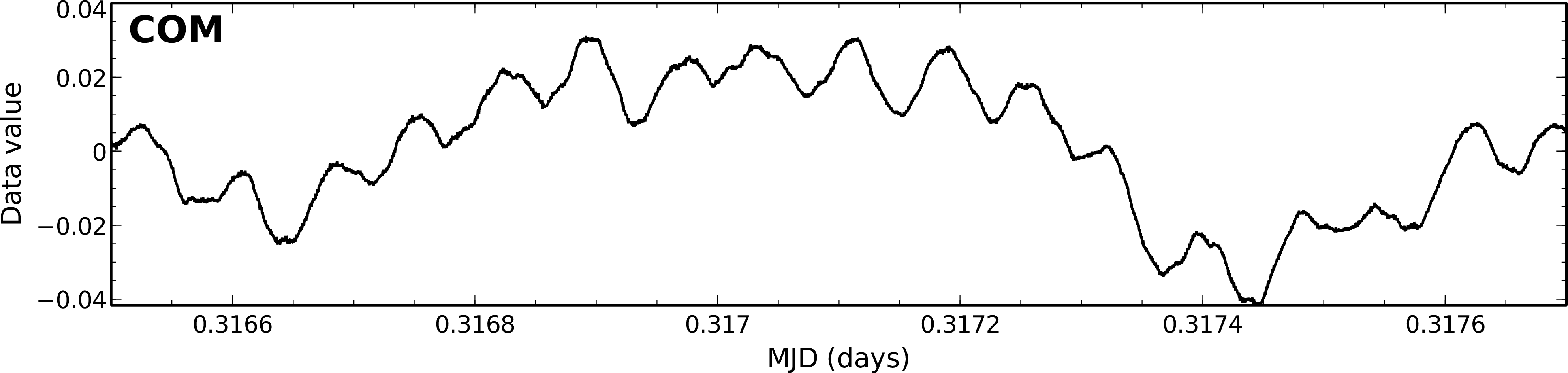
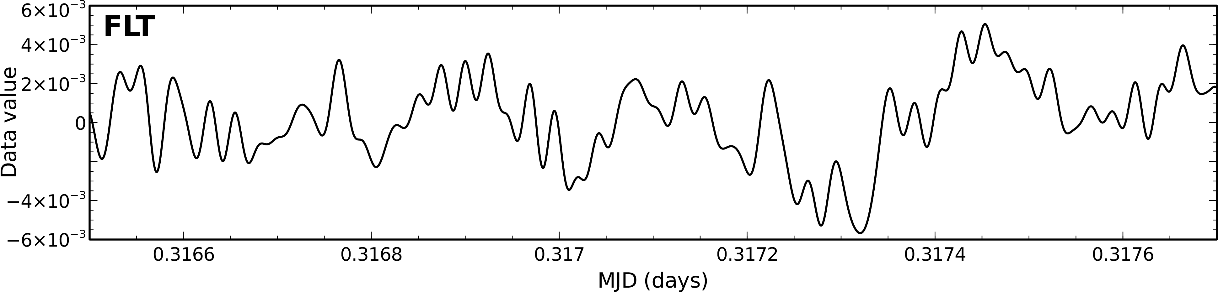
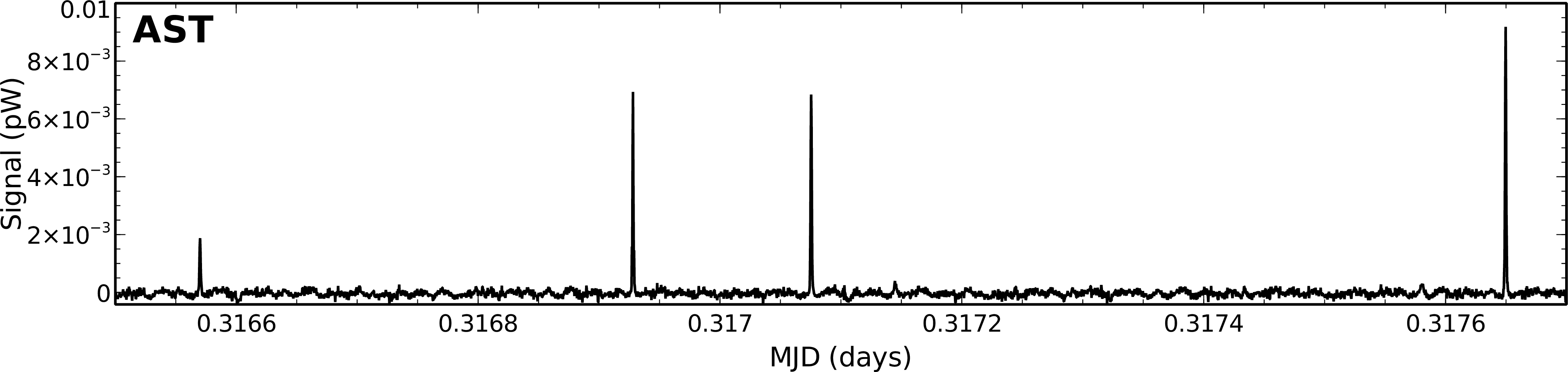
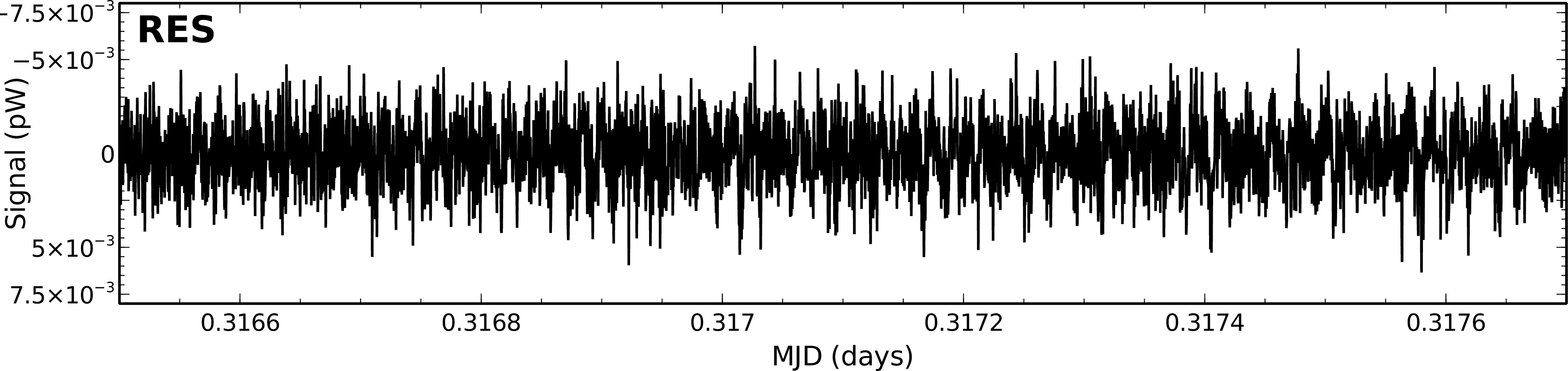
Examples of the time traces for a single bolometer from these models is shown in Figure 3.2. These traces cover
a subset of an observation of the secondary calibrator CRL 2688. You can clearly see the dominance of the COM
model which is removed first. The FLT model stores the data removed by the high-pass filter. In the AST model,
CRL 2688 is clearly seen as positive spikes which appear when the bolometer passes over the source. Finally,
the residual signal stored in RES is flat, indicating that most of the signal has been successfully accounted for by
the other model components.
3.4 Stopping criteria
The map-maker will stop processing either when the requested number of iterations has been completed OR
when the convergence criterion specified in the configuration file is reached.
Option 1: Fixed number of iterations
Specifying the number of iterations in the configuration file is done via the numiter parameter. This is shown
below for dimmconfig_jsa_generic.lis (JSA stands for “JCMT Science Archive”).
A positive value for numiter means that the requested number of iterations will be executed. A negative
value, as in the example above, indicates that no more than this number of iterations should be
performed, but that it may stop at fewer if convergence (according to the noise criterion below) has been
achieved.
Option 2: Convergence parameter
The convergence criterion is set by the maptol parameter.
When running the map-maker, maptol gives the average normalised change in the value of
map pixels between subsequent iterations. Convergence is reached when the mean change
across all pixels is less than the parameter maptol. It has units of the noise in the map, thus
maptol=0.05 means a mean change in pixel value of
<0.05 σ.
This option has the advantage of directly assessing the noise in the resulting map.
The map-maker displays the normalised change in pixel values between iterations at the end of
each iteration. This value typically drops rapidly to begin with and then flattens out, decreasing
increasingly slowly. The printed values can be inspected to check convergence is proceeding as
expected. Be aware that setting maptol to much lower than 0.05 will dramatically increase the
length of time needed to produce the final map, and may possibly result in convergence never being
achieved.
If you wish to perform further checks on the progress of convergence while running the map-maker, you can
use the itermap option. This causes the map created by each iteration to be dumped to disk for inspection (see
Section 6).
3.5 Masking
The term masking refers to the inclusion or exclusion of selected bolometer samples from the estimate of specific
models, based on the positions of those samples within the output map. Masking can be applied
independently to the AST, FLT and COM models, as described in the later sub-sections within this
section.
A mask is a selection of pixels within the output map. Normally these pixels form one or more contiguous
regions that enclose the areas where significant sub-mm emission is expected (the “source” regions). Pixels
outside this mask are referred to as “background pixels”. The use to which such masks are put differs from
model to model as described later in model-specific sub-sections.
Masks fall into two broad categories:
- dynamic masks – these are masks that change shape from one iteration to the next.
- static masks – these are masks that retain the same shape for all iterations.
Static masks are appropriate in cases where the areas containing significant sub-mm emission are
known in advance. If this is not the case, then the mask needs to be based on evidence within the
maps created at the end of each iteration, resulting in the masks evolving from iteration to
iteration as the maps converge towards the final solution. Such dynamic masks have a potential
problem in that they can upset the convergence process by introducing extra flexibility into the
algorithm. For this reason, an option is provided to freeze these masks after a fixed number of
iterations (e.g.
see ast.zero_freeze) and this is used within the specialist configuration file dimmconfig_fix_convergence described
in Section 3.8.
Each of the three models—AST, FLT and COM —have an equivalent set of parameters to specify the masking (if
any) that should be used. Each set starts with the model name, followed by a dot, followed by the parameter
name. To enable masking, one or more of these parameters needs to be set to a suitable value to define a mask,
as described below.
Static masks can be defined either as circles of specified radius, centred on the source position
(suitable for compact sources—see for instance ast.zero_circle), or by an external image that uses
special pixel values to indicate the source regions and the background regions (suitable for extended
sources—see for instance ast.zero_mask). Within such “external masks” all background pixels
should be set to the Starlink bad value (see “Bad-pixel Masking” in SUN/95). Pixels with any other
value are treated as source pixels. Section 6.6 describes some ways in which external masks can be
generated.
Dynamic masks can be defined in several different ways:
-
(1)
- By applying a simple threshold on the S/N ratio within the map created at the end of each iteration
(e.g. see
ast.zero_snr).
-
(2)
- By applying a simple threshold on the S/N ratio as above, and then extending the resulting source
regions down to a lower S/N value (e.g. see
ast.zero_snrlo). This allows a low S/N threshold
to be used (which can sometimes help to avoid negative bowling around the edges of extended
sources) without introducing lots of isolated pixels into the mask because of noise spikes in the
map.
-
(3)
- By applying a threshold on the number of bolometer samples falling in each map pixel (e.g. see
ast.zero_lowhits). Because of the scanning strategy used with SCUBA-2 (see Section 2.2), pixels
near the edge of the map will receive fewer bolometer samples than those near the centre, and will
therefore be noisier. Thus this scheme allows the noisy edges of the map to be masked out. Whilst
this is technically a dynamic mask—because the number of samples falling in each pixel could
potentially change from iteration to iteration—in fact a mask based on hits per pixel will usually
only change very slightly from iteration to iteration.
-
(4)
- By using an algorithm that automatically identifies features of a given size in the map, similar to
that used by the Kappa ffclean command (e.g. see
ast.zero_snr_ffclean). This can be a useful
alternative to simple S/N thresholding in cases where bright artificial large-scale structures appear
in the map. Such structures will result in artificially large source regions in a simple S/N mask,
which may in turn cause the artificial structures to become even brighter and larger in subsequent
iterations. Using an ffclean-based mask instead will restrict the mask to the brighter astronomical
cores on top of such artificial large-scale structures.
Multiple masks can be used by selecting the appropriate configuration parameters as described above. Whether
the combined mask represents the union or intersection of the individual masks is selected using
the parameters ast.zero_union, flt.zero_union and com.zero_union. By default, the union is
used.
The masks used on the last iteration are stored in the Quality component of the NDF containing the output
map. A separate bit of the quality component is used for each model (AST, FLT or COM) that is being masked.
These bits can be viewed in various ways—see Section 8.6 and Section 5.3.2.
Tip: Be aware that the S/N ratio within individual map pixels depends on pixel size—larger pixels will have
higher S/N ratios than small pixels. Therefore masks based on a specific S/N threshold will grow or shrink in
area as a function of pixel size. As a rough rule, if you double the pixel size, you should also double the S/N
thresholds to get a mask that covers a similar area of the sky.
3.5.1 AST masking
The iterative map-maker algorithm described earlier in this chapter divides each cleaned bolometer value into
four additive parts:
-
(1)
- The common-mode signal (
COM).
-
(2)
- The low frequency background drift in each bolometer (
FLT).
-
(3)
- The astronomical signal (
AST).
-
(4)
- The left-over residual noise (
RES).
Whilst the value of each model is constrained to some extent by the manner in which the model is calculated,
there remains a large degree of degeneracy in the algorithm. In other words, there are many different ways in
which each bolometer value can be divided up into the four values listed above. For instance, any arbitrary
change in the AST model can be accommodated provided that equal and opposite changes are
introduced into the other model values so that the total value of all four components remains the
same.
The degeneracy between COM and AST is particularly problematic, since it allows large scale features
to appear in the map (on the scale of the sub-array footprint) that are corrected for by equal and
opposite features in the COM model. Such features can appear as gradients or “saddles” across the final
map.
The purpose of masking the AST model is to apply an extra constraint to the system to help break this
degeneracy, and so avoid these large-scale features. It functions by forcing the AST model to zero at the end of
each iteration for all samples that fall outside the masked area on the sky (i.e. samples that fall in the
“background” areas of the map). Forcing the AST model to zero in this way means that the COM model is more
closely constrained.
Whilst this constraint is applied only in the background regions, its effects are also felt part way into the source
region because of the way in which the COM model averages over a sub-array footprint. Thus source regions that
are much larger than a sub-array will still suffer from the degeneracy between COM and AST, allowing arbitrary
large-scale background features to develop within the region, but these features will become weaker as the
edges of the mask are approached.
In order to avoid the final map containing zero values in the background region, it is necessary to avoid using
AST-masking on the final iteration. For this reason, by default one further iteration is performed—without
AST-masking—once the basic iterative algorithm has converged (see ast.zero_notlast).
All the configuration files supplied with Smurf use AST masking, with the exception of dimmconfig_blank_field.
3.5.2 FLT masking
The FLT model estimates and removes a low frequency background from each bolometer time-stream. To do this
it uses an FFT-based high-pass filter. Ringing around sudden transients—such as astronomical sources — is a
natural consequence of all such filters, resulting in alternating bright and dark rings around sources in the map.
In most cases, the iterative nature of the map-making algorithm eventually results in the rings reducing to a
much lower level, as more of the astronomical signal is removed from the time stream on each iteration, causing
the ring-inducing transients to become weaker. However, this is not always completely effective, and also slows
down convergence.
For these reasons, it is often helpful to mask the FLT model. This causes each bolometer time stream to be
blanked out as the bolometer passes over the source regions in the mask. Such blanked sections are replaced by
linear interpolation between the data on either side of the blanked section. The effect of this is to remove the
transients that cause the ringing in the FLT model, and thus get a better estimate of the low frequency
background in each bolometer.
Such masking is most useful at the start of the iterative process, before the bulk of the astronomical signal has
been removed from the time-streams. Indeed, if it is allowed to continue for too many iterations it can cause its
own problems that tend to slow down convergence. For this reason, if FLT masking is used, it is (by default)
limited to two iterations—see flt.zero_niter.
A difficulty with FLT masking is that the FLT model is evaluated before the map is made on each iteration. This
means that when the FLT model is evaluated on the first iteration, there is no map available. This is not a
problem if a static mask is used, but if a dynamic mask is used, then it is not possible to calculate the FLT mask
on the first iteration (subsequent iterations will create the mask on the basis of the map created at the end of the
previous iteration). This is a shame since FLT masking is most beneficial on the first few iterations, whilst the
bulk of the astronomical signal is still present in the time streams. A scheme to get around this problem is
described in Section 3.6.
All the configuration files supplied with Smurf use FLT masking, with the exception of dimmconfig_blank_field.
3.5.3 COM masking
The value of the COM model at a specific time-slice is the mean of all remaining bolometer values at that time
slice. If the COM model is masked, bolometer samples that fall within the source regions defined by the mask are
excluded from this mean, thus removing the bias introduced into the mean by bright astronomical sources. This
results in the COM model more accurately representing the varying common-mode background value at each
time slice. This can help to reduce negative bowling around sources in the map, and can help to
reduce the amount of data that is rejected as being too poorly correlated with the common-mode
signal.
COM masking has the same difficulty as FLT masking in that the COM model is evaluated before the map is made on
each iteration, and so it is difficult to use dynamic masks with COM masking. However, the solution described in
Section 3.6 can be used for COM masking as for FLT masking.
Currently, none of the configuration files supplied with Smurf use COM masking.
3.6 Skipping the AST model
As discussed in Section 3.5, FLT masking is most effective on the early iterations (particularly the first iteration).
This is because the bulk of the astronomical signal is still present in the time streams and is likely to cause bad
ringing if FLT masking is not used. However, since the FLT model is evaluated before the map is made
within each iteration, there is no map available to use as the basis for a FLT mask on the very first
iteration.
One way to get round this is simply to use a static mask that does not require a map to be available. However,
this may not be possible, particularly for extended sources where no a-priori knowledge of the source areas in
the sub-mm may be available.
Another scheme is provided by the ast.skip configuration parameter. If ast.skip is set to a positive integer
N, the subtraction
of the AST model from the time-series that normally occurs at the end of each iteration is not performed on the first
N iterations. This means
that for the first N
iterations, the time-series data remain unchanged, and consequently the models and the resulting
map are unchanged. Of itself, this does nothing useful—it merely delays the first useful iteration.
However, when combined with FLT masking, it can be very beneficial because it allows a mask to
be created before the first “real” iteration occurs (i.e. the first iteration that subtracts off the AST
model). This means that the first “real” map will have far less ringing around bright sources than
would otherwise be the case. This in turn means that far fewer iterations are required to correct this
ringing.
It is also possible to use ast.skip with COM masking, but the benefits are not so noticeable as for FLT
masking.
The default value for ast.skip is zero, but the dimmconfig_bright_extended and
dimmconfig_jsa_generic configuration files supplied with Smurf both set ast.skip = 5 (and also use FLT
masking).
3.7 Specialised configuration files
Maps made by the pipeline using the REDUCE_SCAN recipe will use dimmconfig_jsa_generic.lis unless
some alternative configuration has been specified. This configuration file is intended to provide a reasonably
good map for all types of observations. However, compromises have been made to reach that balance, the main
one being that some real extended structure is sacrificed in order to avoid introducing artificial large scale
structures.
Whilst dimmconfig_jsa_generic.lis is always a good place to start, you will want to follow this up with a
specialised configuration that will suit your observation. A few specialised configuration files are supplied with
Smurf and can be found in $STARLINK_DIR/share/smurf/.
Note, any parameter for which no value is specified within the supplied configuration will take on the default
value listed in Appendix I.
Below is a description of each of the specialised configuration files. The tables following each description list the
parameters set by each file. The files themselves are stored in $STARLINK_DIR/share/smurf/—they are simple
text files and so can be inspected easily.
3.7.1 dimmconfig_jsa_generic.lis
The dimmconfig_jsa_generic configuration file is designed to handle all science data. This is a good
configuration file to start with if you are unsure how to proceed with your data reduction. You
may notice that elements of this configuration are common to the other specialised configuration
files.
This configuration is optimised to suppress the creation of artificial large scale structure within the final map.
Consequently, some real extended emission may be lost if this configuration is used. This goal is achieved
by:
-
(1)
- Setting
flt.filt_edge_largescale) to 200 arcseconds so that the FLT model uses a heavier than
normal filter.
-
(2)
- Setting
com.perarray to 1, indicating that four separate COM models should be used, one for each
sub-array.
-
(3)
- Using a mask to force the
AST model to zero in the background regions after each iteration (see
parameters ast.zero_snr and ast.zero_snrlo—also see Section 3.5.1).
In addition the S/N threshold for DC steps (dcthresh) is relaxed from 25 in the default file to 100 to avoid
problems bright sources triggering the step detection algorithm.
The other major feature of this configuration is that the subtraction of the AST model is skipped on the first five
iterations. In conjunction with the use of FLT masking, this helps to speed up convergence and minimise dark
rings around bright source (see Section 3.6.
3.7.2 dimmconfig_blank_field.lis
The dimmconfig_blank_field configuration is tuned for blank field surveys for which the goal is to detect
extremely low signal-to-noise point sources within otherwise blank fields.
Applying a high-pass filter (FLT) on each iteration can result in convergence problems when there is little or no signal in
the map. Instead, a single, harsher high-pass filter is applied as a pre-processing step (corresponding to 200-arcsec scales
at both 450 μm
and 850 μm).
There are also more conservative cuts to remove noisy/problematic bolometers. Only 4 (positive) iterations are
requested as there is no signal to confuse to models.
The option com.perarray = 1 requires the COM model to be fit to each sub-array independently. This improves
the overall fit but with the loss of any structure on scales larger than a single sub-array—not an issue for blank
fields.
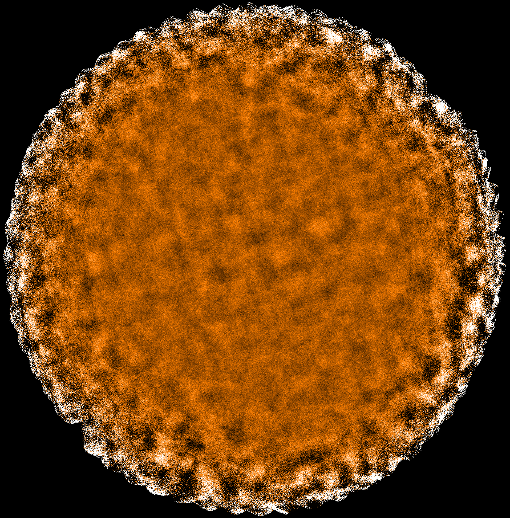
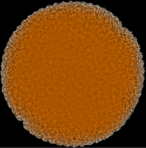
Figure 3.3 shows the sharp contrast in the output map between reducing data with the default configuration
file and using dimmconfig_blank_field.lis.
Blank-field maps commonly have a matched filter applied as part of the post-processing to aid source detection
(see Section 8.7), however this is not applied by the map-maker.
3.7.3 dimmconfig_bright_compact.lis
The dimmconfig_bright_compact configuration should be used for producing maps of bright, isolated
compact sources that are positioned at the centre of the map (e.g. calibrators).
The addition of the ast.zero_circle parameter is used to constrain the map to zero beyond a radius of
1 arc-min from the source centre (see Section 3.5.1). This strategy helps with map convergence significantly, and
can provide good maps of bright sources, even in cases where scan patterns failed to complete in
full.
com.perarray is set to 1 indicating that a COM model should be fit separately for each sub-array. This is not
advised for extended sources as signal on scales larger than a single sub-array is lost, but is fine
for a compact central source. Likewise, the filtering is tighter. The S/N threshold for DC steps
(dcthresh) is relaxed from 25 in the default file to 100 to avoid problems associated with bright
sources.
The values of the parameters controlling the COM model are modified to relax the test that compares each
bolometer to the common mode. This is because the algorithm that compares each bolometer to the
common-mode can be fooled by a bright compact source passing across individual bolometers. Likewise the test
for DC steps within each bolometer baseline is also relaxed (parameter dcthresh).
3.7.4 dimmconfig_bright_extended.lis
The dimmconfig_bright_extended configuration is for reducing maps that contain emission that is extended
to some degree and contains some bright regions. Here, the combination of ast.zero_snr and
ast.zero_snrlo is used to identify components of the AST model wherever the S/N is higher than
3σ and then to expand this basic
mask down to an SNR equal to 2σ
without introducing any new isolated source areas (see Section 3.5.1). numiter has been raised to -40,
as more iterations are required to maximise the sensitivity to large dynamic signal ranges in the
map.
The other major feature of this configuration is that the subtraction of the AST model is skipped on the first five
iterations. In conjunction with the use of FLT masking, this helps to speed up convergence and minimise dark
bowls around bright source (see Section 3.6.
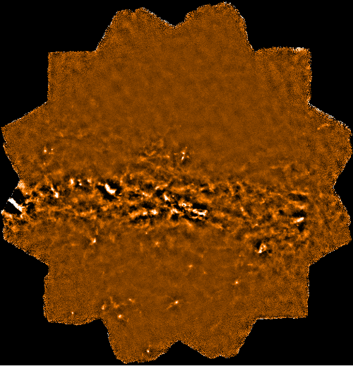
Figure 3.4 shows a comparison between maps reduced with the default configuration file and using
dimmconfig_bright_extended.lis; the most noticeable difference is the improvement in the bowling around
strong sources.
3.7.5 dimmconfig_pca.lis
The newest dimmconfig file (2019) is called: dimmconfig_pca.lis. This parameter file can be combined with
other dimmconfig files to tell makemap to include a Principal Component Analysis (PCA) model in its iterative
algorithm (the PCA model removes noise signals that are correlated between multiple bolometer time-streams).
For instance, to use a PCA model when creating a map of a bright extended source, you could run makemap as
follows:
% more conf
^$STARLINK_DIR/share/smurf/dimmconfig_bright_extended.lis
^$STARLINK_DIR/share/smurf/dimmconfig_pca.lis
% makemap config=^conf
To process compact sources, change “bright_extended” above to “bright_compact“.
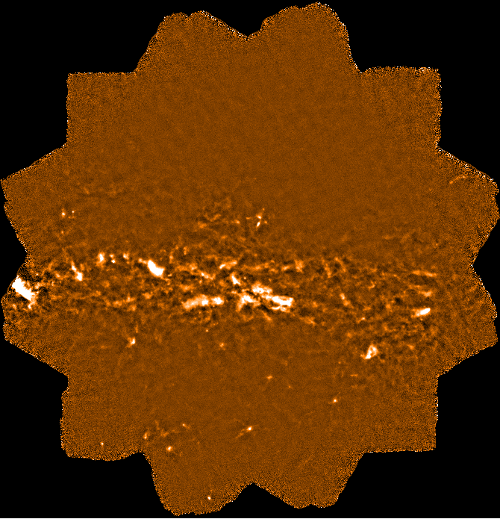
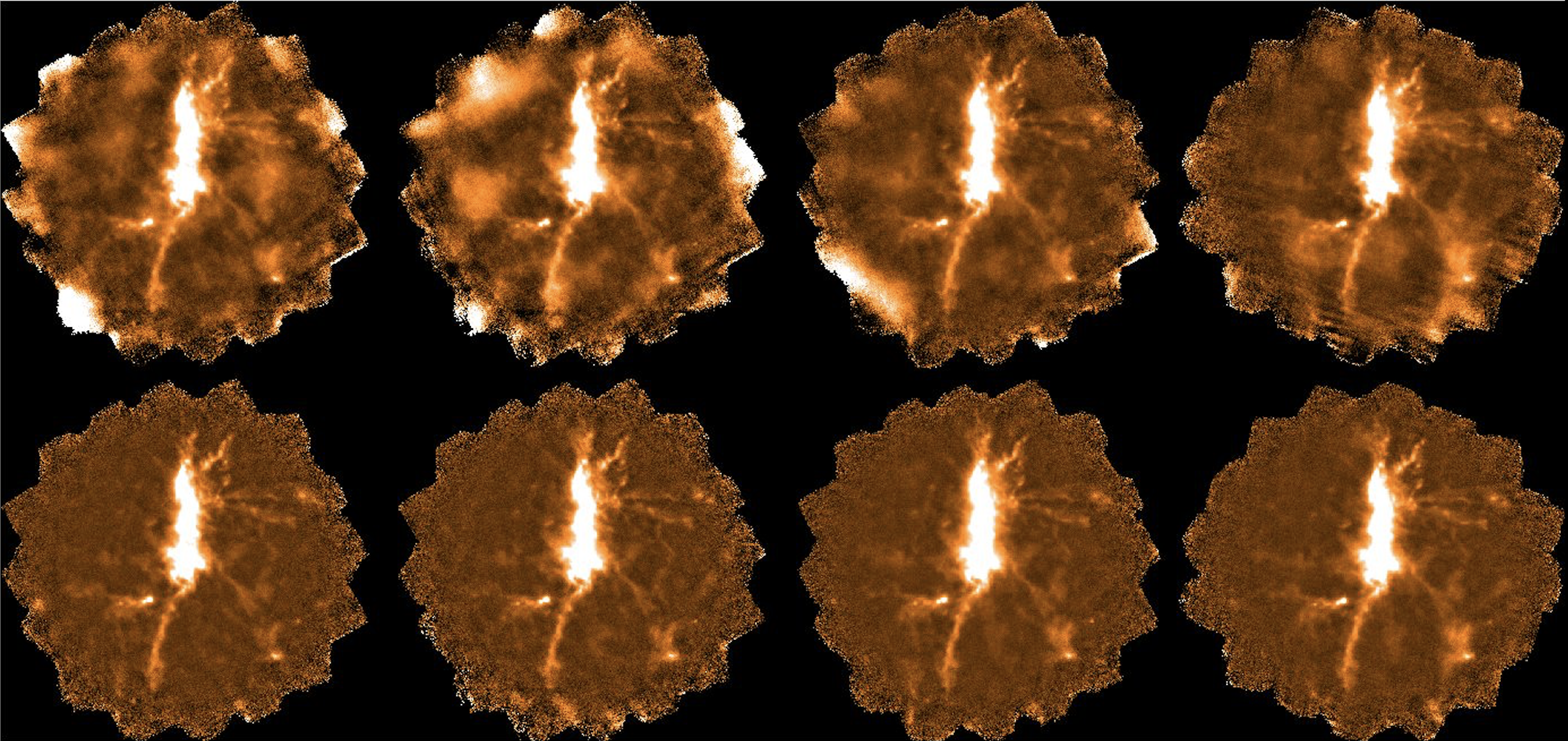
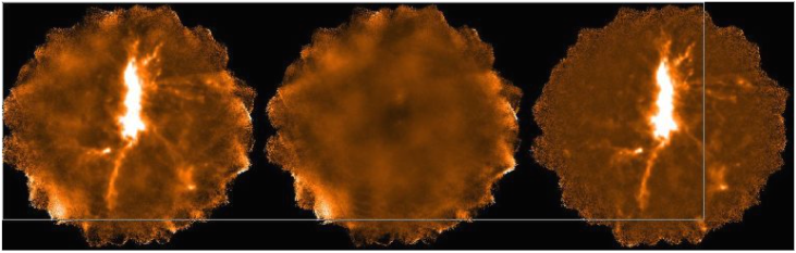
Using a PCA model can help to reduce the spurious extended structures that often appear in SCUBA-2
maps (although this benefit is bought at the cost of a much extended run time). For instance, four
850-μm
maps of DR 21 are presented in Figure 3.5. Its top row shows the maps made with the basic “bright
extendedd” dimmconfig, the middle row shows the results of adding in the new PCA dimmconfig, and the
bottom row shows mosaics of the top and middle rows (left and right, respectively) with a difference map in
between.
3.8 Configuration files for solving specific problems
Two additional configuration files are available that can be used to supplement your configuration file in order
to solve specific problems:
dimmconfig_fix_convergence to help your map converge. It does this by preventing masks from
changing, and by freezing the flags that identify aberrant bolometers. Both of these restrictions are
imposed only after 10 iterations have been performed.
dimmconfig_fix_blobs to remove large “blooms” or smooth blobs of spurious emission in your
map. These can be caused by ringing induced by unidentified steps or spikes in the bolometer
time-streams. The fix is to look for oscillations within the time-streams following the FLT model,
and flag such time-slices as unusable. In addition, time slices at which the four sub-arrays see
significantly different common-mode values are also flagged as unusable.
These files provide a few additional settings that should be added to some other configuration in order to
achieve the desired fix. For instance, a configuration file containing the following two lines would indicate that
values from both dimmconfig_bright_extended.lis and dimmconfig_fix_blobs.lis should be
used:
^/star/share/smurf/dimmconfig_bright_extended.lis
^/star/share/smurf/dimmconfig_fix_blobs.lis
This reads a set of configuration parameter from the dimmconfig_bright_extended.lis file, and then assigns
new values for just those parameters defined in dimmconfig_fix_blobs.lis. These values override the values
specified in dimmconfig_bright_extended.lis.
The parameters in these files are discussed further Chapter 6.
Copyright © 2014-2021 Science and Technology Facilities Council,
East Asian Observatory