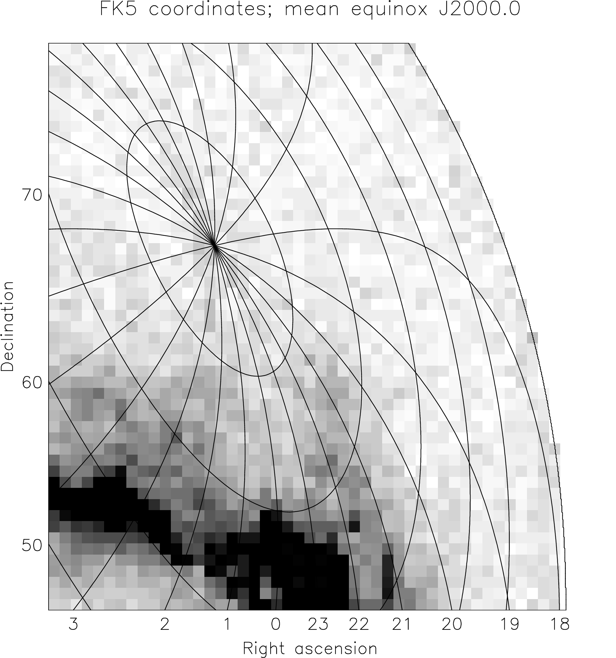
Figure 9: An example of a displayed image with a coordinate grid plotted over it.
For those of you with a plane to catch, this section provides some instant templates and recipes for performing the most commonly-required operations using AST, but without going into detail. The examples given (sort of) follow on from each other, so you should be able to construct a variety of programs by piecing them together. Note that some of them appear longer than they actually are, because we have included plenty of comments and a few options that you probably won’t need.
If any of this material has you completely baffled, then you may want to read the introduction to AST programming concepts in §4 first. Otherwise, references to more detailed reading are given after each example, just in case they don’t quite do what you want.
The AST library is available both as a stand-alone package and also as part of the Starlink Software Collection4. If your site has the Starlink Software Collection installed then AST should already be available.
If not, you can download the AST library by itself from http://www.starlink.ac.uk/ast/.
An AST program normally has the following structure:
The use of astBegin and astEnd is optional, but has the effect of tidying up after you have finished using AST, so is normally recommended. For more details of this, see §4.10. For details of how to access the “ast.h” header file, see §22.1.
To build a simple AST program that doesn’t use graphics, use:
To build a program which uses PGPLOT for graphics, use:
For more details about accessing the “ast.h” header file, see §22.1. For more details about linking programs, see §22.2 and the description of the “ast_link” command in Appendix E.
Precisely how you extract world coordinate system (WCS) information from a dataset obviously depends on what type of dataset it is. Usually, however, you should be able to obtain a set of FITS header cards which contain the WCS information (and probably much more besides). Suppose that “cards” is a pointer to a string containing a complete set of concatenated FITS header cards (such as produced by the CFITSIO function fits_hdr2str). Then proceed as follows:
The result should be a pointer, “wcsinfo”, to a FrameSet which contains the WCS information. This pointer can now be used to perform many useful tasks, some of which are illustrated in the following recipes.
Some datasets which do not easily yield FITS header cards may require a different approach, possibly involving use of a Channel or XmlChan (§15) rather than a FitsChan. In the case of the Starlink NDF data format, for example, all the above may be replaced by a single call to the function ndfGtwcs—see SUN/33. The whole process can probably be encapsulated in a similar way for most data systems, whether they use FITS header cards or not.
For more details about reading WCS information from datasets, see §17.3 and §17.4. For a more general description of FitsChans and their use with FITS header cards, see §16 and §17. For more details about FrameSets, see §13 and §14.
Once you have read WCS information from a dataset, as in §3.4, you may wish to check that you have been successful. The following will detect and classify the things that might possibly go wrong:
For more information about detecting errors in AST functions, see §4.15. For details of how to validate input data read by AST, see §15.6 and §17.4.
If you have a pointer to any AST Object, you can display the data stored in that Object in textual form as follows:
Here, we have used a pointer to the FrameSet which we read earlier (§3.4). The result is written to the program’s standard output stream. This can be very useful during debugging.
For more details about using astShow, see §4.4. For information about interpreting the output, also see §15.8.
You may use a pointer to a FrameSet, such as we read in §3.4, to transform a set of points between the pixel coordinates of an image and the associated world coordinates. If you are working in two dimensions, proceed as follows:
Here, N is the number of points to be transformed, “xpixel” and “ypixel” hold the pixel coordinates, and “xworld” and “yworld” receive the returned world coordinates.5 To transform in the opposite direction, interchange the two pairs of arrays (so that the world coordinates are given as input) and change the fifth argument of astTran2 to zero.
To transform points in one dimension, use astTran1. In any other number of dimensions (or if the number of dimensions is initially unknown), use astTranN or astTranP. These functions are described in Appendix B.
For more information about transforming coordinates, see §4.8 and §13.6. For details of how to handle missing coordinates, see §5.9.
The world coordinate system (WCS) currently associated with an image may often be a celestial coordinate system, but this need not necessarily be the case. For instance, instead of right ascension and declination, an image might have a WCS with axes representing wavelength and slit position, or maybe just plain old pixels.
If you have obtained a WCS calibration for an image, as in §3.4, in the form of a pointer “wcsinfo” to a FrameSet, then you may determine if the current coordinate system is a celestial one or not, as follows:
This will set “issky” to 1 if the WCS is a celestial coordinate system, and to zero otherwise.
Testing for a spectral coordinate system is basically the same as testing for a celestial coordinate system (see the previous section). The one difference is that you use the astIsASpecFrame function in place of the astIsASkyFrame function.
Once you have converted pixel coordinates into world coordinates (§3.7), you may want to format them as text before displaying them. Typically, this would convert from (say) radians into something more comprehensible. Using the FrameSet pointer “wcsinfo” obtained in §3.4 and a pair of world coordinates “xw” and “yw” (e.g. see §3.7), you could proceed as follows:
Here, the second argument to astFormat is the axis number.
With celestial coordinates, this will usually result in sexagesimal notation, such as “12:34:56.7”. However, the same method may be applied to any type of coordinates and appropriate formatting will be employed.
For more information about formatting coordinate values and how to control the style of formatting used, see §7.6 and §8.6. If necessary, also see §7.7 for details of how to “normalise” a set of coordinates so that they lie within the standard range (e.g. 0 to 24 hours for right ascension and ±90∘ for declination).
In addition to formatting coordinates as part of a program’s output, you may also want to examine coordinate values while debugging your program. To save time, you can “eavesdrop” on the coordinate values being processed every time they are transformed. For example, when using the FrameSet pointer “wcsinfo” obtained in §3.4 to transform coordinates (§3.7), you could inspect the coordinate values as follows:
By setting the FrameSet’s Report attribute to 1, coordinate transformations are automatically displayed on the program’s standard output stream, appropriately formatted, for example:
For a complete description of the Report attribute, see its entry in Appendix C. For further details of how to set and enquire attribute values, see §4.6 and §4.5.
In addition to writing out coordinate values generated by your program (§3.10), you may also need to accept coordinates entered by a user, or perhaps read from a file. In this case, you will probably want to allow “free-format” input, so that the user has some flexibility in the format that can be used. You will probably also want to detect any typing errors.
Let’s assume that you want to read a number of lines of text, each containing the world coordinates of a single point, and to split each line into individual numerical coordinate values. Using the FrameSet pointer “wcsinfo” obtained earlier (§3.4), you could proceed as follows:
This algorithm has the advantage of accepting free-format input in whatever style is appropriate for the world coordinates in use (under the control of the FrameSet whose pointer you provide). For example, wavelength values might be read as floating point numbers (e.g. “1.047” or “4787”), whereas celestial positions could be given in sexagesimal format (e.g. “12:34:56” or “12 34.5”) and would be converted into radians. Individual coordinate values may be separated by white space and/or any non-ambiguous separator character, such as a comma.
For more information on reading coordinate values using the astUnformat function, see §7.8. For details of how sexagesimal formats are handled, and the forms of input that may be used for celestial coordinates, see §8.7.
This section describes how to add a WCS calibration to a data set which you are creating from scratch, rather than modifying an existing data set.
In most common cases, the simplest way to create a new WCS calibration from scratch is probably to create a set of strings describing the required calibration in terms of the keywords used by the FITS WCS standard, and then convert these strings into an AST FrameSet describing the calibration. This FrameSet can then be used for many other purposes, or simply stored in the data set.
The full FITS-WCS standard is quite involved, currently running to four separate papers, but the basic kernel is quite simple, involving the following keywords (all of which end with an integer axis index, indicated below by <i>):
As an example consider the common case of a simple 2D image of the sky in which north is parallel to the second pixel axis and east parallel to the (negative) first pixel axis. The image scale is 1.2 arc-seconds per pixel on both axes, and the image is presumed to have been obtained with a tangent plane projection. Furthermore, it is known that pixel coordinates (100.5,98.4) correspond to an RA of 11:00:10 and a Dec. of -23:26:02. A suitable set of FITS-WCS header cards could be:
Notes:
The EQUINOX value defaults to J2000.0 if omitted. FK4 can also be used in place of FK5, in which case EQUINOX defaults to B1950.0.
Once you have created these FITS-WCS header card strings, you should store them in a FitsChan and then read the corresponding FrameSet from the FitsChan. How to do this is described in §3.4.
Having created the WCS calibration, you may want to store it in a data file. How to do this is described in §3.15).6
If the required WCS calibration cannot be described as a set of FITS-WCS headers, then a different approach is necessary. In this case, you should first create a Frame describing pixel coordinates, and store this Frame in a new FrameSet. You should then create a new Frame describing the world coordinate system. This Frame may be a specific subclass of Frame such as a SkyFrame for celestial coordinates, a SpecFrame for spectral coordinates, a Timeframe for time coordinates, or a CmpFrame for a combination of different coordinates. You also need to create a suitable Mapping which transforms pixel coordinates into world coordinates. AST provides many different types of Mappings, all of which can be combined together in arbitrary fashions to create more complicated Mappings. The WCS Frame should then be added into the FrameSet, using the Mapping to connect the WCS Frame with the pixel Frame.
The usual reason for wishing to modify the WCS calibration associated with a dataset is that the data have been geometrically transformed in some way (here, we will assume a 2-dimensional image dataset). This causes the image features (stars, galaxies, etc.) to move with respect to the grid of pixels which they occupy, so that any coordinate systems previously associated with the image become invalid.
To correct for this, it is necessary to set up a Mapping which expresses the positions of image features in the new data grid in terms of their positions in the old grid. In both cases, the grid coordinates we use will have the first pixel centred at (1,1) with each pixel being a unit square.
AST allows you to correct for any type of geometrical transformation in this way, so long as a suitable Mapping to describe it can be constructed. For purposes of illustration, we will assume here that the new image coordinates “xnew” and “ynew” can be expressed in terms of the old coordinates “xold” and “yold” as follows:
where “m” is a 2×2 transformation matrix and “z” represents a shift of origin. This is therefore a general linear coordinate transformation which can represent displacement, rotation, magnification and shear.
In AST, it can be represented by concatenating two Mappings. The first is a MatrixMap, which implements the matrix multiplication. The second is a WinMap, which linearly transforms one coordinate window on to another, but will be used here simply to implement the shift of origin (alternatively, a ShiftMap could have been used in place of a WinMap). These Mappings may be constructed and concatenated as follows:
You might, of course, create any other form of Mapping depending on the type of geometrical transformation involved. For an overview of the Mappings provided by AST, see §2.2, and for a description of the capabilities of each class of Mapping, see its entry in Appendix D. For an overview of how individual Mappings may be combined, see §2.3 (§6 gives more details).
Assuming you have obtained a WCS calibration for your original image in the form of a pointer to a FrameSet, “wcsinfo1” (§3.4), the Mapping created above may be used to produce a calibration for the new image as follows:
This will produce a pointer, “wcsinfo2”, to a new FrameSet in which all the coordinate systems associated with your original image are modified so that they are correctly registered with the new image instead.
For more information about re-mapping the Frames within a FrameSet, see §14.4. Also see §14.5 for a similar example to the above, applicable to the case of reducing the size of an image by binning.
If you have modified the WCS calibration associated with a dataset, such as in the example above (§3.14), then you will need to write the modified version out along with any new data.
In the same way as when reading a WCS calibration (§3.4), how you do this will depend on your data system, but we will assume that you wish to generate a set of FITS header cards that can be stored with the data. You should usually make preparations for doing this when you first read the WCS calibration from your input dataset by modifying the example given in §3.4 as follows:
Note how we have added an enquiry to determine how the WCS information is encoded in the input FITS cards, storing a pointer to the resulting string in the “encode” variable. This must be done before actually reading the WCS calibration.
(N.B. If you will be making extensive use of astGetC in your program, then you should allocate a buffer and make a copy of this string, because the pointer returned by astGetC will only remain valid for 50 invocations of the function, and you will need to use the Encoding value again later on.)
Once you have produced a modified WCS calibration for the output dataset (e.g. §3.14), in the form of a FrameSet identified by the pointer “wcsinfo2”, you can produce a new FitsChan containing the output FITS header cards as follows:
For details of how to modify the contents of the output FitsChan in other ways, such as by adding, over-writing or deleting header cards, see §16.4, §16.9, §16.8 and §16.13.
Once you have assembled the output FITS cards, you may retrieve them from the FitsChan that contains them as follows:
Here, we have simply written each card to the standard output stream, but you would obviously replace this with a function invocation to store the cards in your output dataset.
For data systems that do not use FITS header cards, a different approach may be needed, possibly involving use of a Channel or XmlChan (§15) rather than a FitsChan. In the case of the Starlink NDF data format, for example, all of the above may be replaced by a single call to the function ndfPtwcs—see SUN/33. The whole process can probably be encapsulated in a similar way for most data systems, whether they use FITS header cards or not.
For an overview of how to propagate WCS information through data processing steps, see §17.6. For more information about writing WCS information to FitsChans, see §16.5 and §17.7. For information about the options for encoding WCS information in FITS header cards, see §16.1, §17.1, and the description of the Encoding attribute in Appendix C. For a complete understanding of FitsChans and their use with FITS header cards, you should read §16 and §17.
A common requirement when displaying image data is to plot an associated coordinate grid (e.g. Figure 9) over the displayed image.
The use of AST in such circumstances is independent of the underlying graphics system, so starting up the graphics system, setting up a coordinate system, displaying the image, and closing down afterwards can all be done using the graphics functions you would normally use.
However, displaying an image at a precise location can be a little fiddly with some graphics systems, and obviously the grid drawn by AST will not be accurately registered with the image unless this is done correctly. In the following template, we therefore illustrate both steps, basing the image display on the C interface to the PGPLOT graphics package.7 Plotting a coordinate grid with AST then becomes a relatively minor part of what is almost a complete graphics program.
Once again, we assume that a pointer, “wcsinfo”, to a suitable FrameSet associated with the image has already been obtained (§3.4).
Note that once you have set up a Plot which is aligned with a displayed image, you may also use it to generate further graphical output of your own, specified in the image’s world coordinate system (such as markers to represent astronomical objects, annotation, etc.). There is also a range of Plot attributes which gives control over most aspects of the output’s appearance. For details of the facilities available, see §21 and the description of the Plot class in Appendix D.
For details of how to build a graphics program which uses PGPLOT, see §3.3 and the description of the ast_link command in Appendix E.
Once you have set up a Plot to draw a coordinate grid (§3.16), it is a simple matter to change things so that the grid represents a different celestial coordinate system. For example, after creating the Plot with astPlot, you could use:
or:
and any axes and/or grid drawn subsequently would represent the new celestial coordinate system you specified. Note, however, that this will only work if the original grid represented celestial coordinates of some kind (see §3.8 for how to determine if this is the case8). If it did not, you will get an error message.
For more information about the celestial coordinate systems available, see the descriptions of the System, Equinox and Epoch attributes in Appendix C.
The idea of using a Plot’s attributes to control the appearance of the graphical output it produces (§3.16 and §3.17) can easily be extended to allow the user of a program complete control over such matters.
For instance, if the file “plot.config” contains a series of plotting options in the form of Plot attribute assignments (see below for an example), then we could create a Plot and implement these assignments before producing the graphical output as follows:
Notice that we take care that the Plot’s Base attribute is preserved so that the user cannot change it. This is because graphical output will not be produced successfully if the base Frame does not describe the plotting surface to which we attached the Plot when we created it.
The arrangement shown above allows the contents of the “plot.config” file to control most aspects of the graphical output produced (including the coordinate system used; the colour, line style, thickness and font used for each component; the positioning of axes and tick marks; the precision, format and positioning of labels; etc.) via assignments of the form:
For a more sophisticated interface, you could obviously perform pre-processing on this input—for example, to translate words like “red”, “green” and “blue” into colour indices, to permit comments and blank lines, etc.
For a full list of the attributes that may be used to control the appearance of graphical output, see the description of the Plot class in Appendix D. For a complete description of each individual attribute (e.g. those above), see the attribute’s entry in Appendix C.
4The Starlink Software Collection can be downloaded from http://www.starlink.ac.uk/Download/.
5By pixel coordinates, we mean a coordinate system in which the first pixel in the image is centred on (1,1) and each pixel is a unit square. Note that the world coordinates will not necessarily be celestial coordinates, but if they are, then they will be in radians.
6If you are writing the WCS calibration to a FITS file you obviously have the choice of storing the FITS-WCS cards directly.
7An interface is provided with AST that allows it to use PGPLOT (SUN/15) for its graphics, although interfaces to other graphics systems may also be written.
8Note that the methods applied to a FrameSet may be used equally well with a Plot.