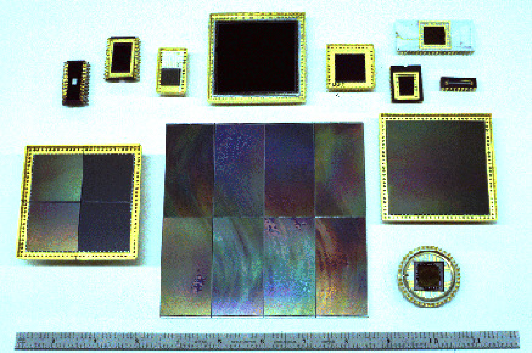
Figure 1: Examples of various CCD chips
Before the introduction of photography to astronomy the only way of recording images of extended objects seen through a telescope was to sketch them. This approach worked moderately well for the planets, which are illuminated by reflected light, but was much less successful for nebulæ and other objects beyond the solar system, both because they are much fainter and because of the inherent difficulty in reproducing the gradations in brightness of an extended luminous object using drawing techniques. Photographic plates were first used to record images of regions of the sky around the middle of the nineteenth century. The techniques proved successful and photographic plates were ubiquitous in astronomy for more than a century. The advantages that they offered were basically threefold:
Nonetheless there were problems with photographic plates: they had only a limited dynamic range and their response to the brightness of the illuminating light was non-linear, leading to persistent calibration problems. In the middle years of the twentieth century photoelectric photometers were developed: electronic devices which were more sensitive, accurate, linear and had a wider dynamic range than the photographic plate. However, they were not imaging devices: they merely produced a single output corresponding to the brightness of one point on the sky.
In many ways CCDs (Charge-Couple Devices) combine the advantages of both photographic plates and photoelectric photometers, though their principles of operation are very different from either. They have a high sensitivity, linear response, large dynamic range and are imaging devices which record a picture of the region of sky being viewed. (Imaging devices are sometimes called, perhaps somewhat grandiloquently, panoramic detectors.)
The CCD was invented in 1969 by W.S. Boyle and G.E. Smith of the Bell Laboratory. They were not interested in astronomical detectors (and were, in fact, investigating techniques for possible use in a ‘picture-phone’). Indeed, most of the applications of CCDs are not astronomical. CCDs were first used in astronomy in 1976 when J. Janesick and B. Smith obtained images of Jupiter, Saturn and Uranus using a CCD detector attached to the 61-inch telescope on Mt Bigelow in Arizona. CCDs were rapidly adopted in astronomy and are now ubiquitous: they are easily the most popular and widespread imaging devices used at optical and near infrared wavelengths.
A CCD is best described as a semiconductor chip, one face of which is sensitive to light (see Figure 1). The light sensitive face is rectangular in shape and subdivided into a grid of discrete rectangular areas (picture elements or pixels) each about 10-30 micron across. The CCD is placed in the focal plane of a telescope so the the light-sensitive surface is illuminated and an image of the field of sky being viewed forms on it. The arrival of a photon on a pixel generates a small electrical charge which is stored for later read-out. The size of the charge increases cumulatively as more photons strike the surface: the brighter the illumination the greater the charge. This description is the merest outline of a complicated and involved subject. For further details see some of the references in Section 2 or the web pages on CCD construction maintained by the University of Oregon. The CCD pixel grids are usually square and the number of pixels on each side often reflects the computer industry’s predilection for powers of two. Early CCDs used in the 1970s often had 6464 elements. 256256 or 512512-element chips were typical in the 1980s and 10241024 or 20482048-element chips are common now.
A CCD in isolation is just a semiconductor chip. In order to turn it into a usable astronomical instrument it needs to be connected to some electronics to power it, control it and read it out. By using a few clocking circuits, an amplifier and a fast analogue-to-digital converter (ADC), usually of 16-bit accuracy, it is possible to estimate the amount of light that has fallen onto each pixel by examining the amount of charge it has stored up. Thus, the charge which has accumulated in each pixel is converted into a number. This number is in arbitrary ‘units’ of so-called ‘analogue data units’ (ADUs); that is, it is not yet calibrated into physical units. The ADC factor is the constant of proportionality to convert ADUs into the amount of charge (expressed as a number of electrons) stored in each pixel. This factor is needed during the data reduction and is usually included in the documentation for the instrument. The chip will usually be placed in an insulating flask and cooled (often with liquid nitrogen) to reduce the noise level and there will be the usual appurtenances of astronomical instruments: shutters, filter wheels etc. The whole instrument is often referred to as a CCD camera. Other synonyms sometimes encountered are area photometer, panoramic photometer or array photometer.
The electronics controlling the CCD chip are interfaced to a computer which in turn controls them. Thus, the images observed by the CCD are transferred directly to computer memory, with no intermediate analogue stage, whence they can be plotted on an image display device or written to magnetic disk or tape. Normally you will return from an observing run with a magnetic tape cartridge of some sort containing copies of the images that you observed.
The principal advantages of CCDs are their sensitivity, dynamic range and linearity. The sensitivity, or quantum efficiency, is simply the fraction of photons incident on the chip which are detected. It is common for CCDs to achieve a quantum efficiency of about 80%. Compare this figure with only a few percent for even sensitised photographic plates. CCDs are also sensitive to a broad range of wavelengths and are much more sensitive to red light than either photographic plates or the photomultiplier tubes used in photoelectric photometers (see Figure 2). However, they have a poor response to blue and ultra-violet light.

CCDs are sensitive to a wide range of light levels: a typical dynamic range (that is, the ratio of the brightest accurately detectable signal to the faintest) is about , corresponding to a range of about 14.5 magnitudes. The corresponding figures for a photographic plate are a range of less than about 1000 corresponding to 7.5 magnitudes. Furthermore, within this dynamic range the response is essentially linear: the size of the signal is simply proportional to the number of photons detected, which makes calibration straightforward.
The principal disadvantage of CCDs is that they are physically small and consequently can image only a small region of sky. Typical sizes are 1.0 to 7.5 cm across, much smaller than photographic plates. There is a practical limit to the size of CCDs because of the time required to read them out. Thus, in order to image a large area of sky it is usual to place several chips in a grid (or mosaic) in the focal plane rather than fabricating a single enormous chip. The large CCD in the foreground in Figure 1 is actually a mosaic of eight chips.
In images observed close to the optical axis of a well-designed telescope an angular displacement on the sky is simply proportional to a linear displacement in position in the focal plane. The constant of proportionality is usually called the plate scale (a name which betrays its origin in photographic techniques) and is traditionally quoted in units of seconds of arc / mm. That is:
| (1) |
where is the plate scale in seconds of arc / mm, is a displacement on the sky in seconds of arc and is the corresponding displacement in the focal plane in mm. If you know the plate scale and the size of either a single pixel in the grid or the linear size of the CCD then it is trivial to use Equation 1 to work out either the angle on the sky subtended by a single pixel or the field of view of the CCD respectively. For example, the sample data used in Part II of the cookbook were obtained with the Jacobus Kapteyn Telescope (JKT) on La Palma. The CCD detector used has pixels which are 2424 micron in size. The plate scale of the JKT is 13.8 seconds of arc / mm. Thus, each pixel subtends an angle of 0.3310.331 seconds of arc on the sky.
The manual for the instrument or telescope that you are using will usually quote a value for the plate scale. However, if necessary it can be calculated from other parameters for the telescope. By simple geometry the plate scale is the reciprocal of the effective focal length of the system:
| (2) |
where is the effective focal length of the system and is the plate scale in units of ‘radians / whatever units is in’. Thus, for in metres and applying the factor for converting radians to seconds of arc:
| (3) |
is itself related to the diameter of the primary mirror, , and the focal ratio, :
| (4) |
At larger distances from the optical axis there is no longer a simple linear relation between angular displacement on the sky and displacement in position in the focal surface. That is, varies as a function of position in the focal surface. This effect is usually not important in instruments containing a single chip because of the small size of individual CCDs. However it may be important if a grid of chips is used.