3 A More Complete Introduction to SPECX

SPECX should be run on a graphics-capable terminal for full use of its capabilities; at the JCMT and elsewhere the preferred device is a Sun workstation. Alternatives are other Xwindow devices (such as DECstation 4000’s and VXT2000’s) and ‘dumb terminals’ like VT330’s. Plot display can be redirected as required to these devices. If you don’t want to plot you can run SPECX on a non-graphics terminal (e.g. a VT220).

3.1 Finding your data

SPECX can read data from data directories that are distinct from your working directory. This leads to directories that are far less cluttered than would otherwise be the case. SPECX does this by using the DATADIR environment variable. When a read-gsd-data or read-gsd-raster command is issued SPECX searches for the GSD file in the current directory and, if the file can not be found, then in the directory specified by DATADIR.

For example, if you stored your data in /data/jcmtrun then you would issue the following command before starting SPECX:

Now when SPECX is started, the directory /data/jcmtrun will be used as a GSD data directory. You are then ready to start up SPECX.

3.2 Getting into SPECX

After you have found your data, and optionally re-directed the plot output (above), give the following command:

which will start up SPECX, setting standard variables and the like. The margin prompt for SPECX commands $>>$ will replace the cshell % prompt, or whatever prompt has been set up:

$>>$

3.3 Things to know about SPECX

There are a few basic principles and tricks which need to be introduced straight away:

• The commands

  $>>$ exit or quit

  get you out of SPECX, returning you to the shell prompt.

• You can abbreviate commands. For example, set-plot-device can be abbreviated to s-p-d. If the command you give is ambiguous you will have to supply more letters. In this guide I will usually give the abbreviated command and perhaps also tell you the full version. If you are unsure of the exact form of a command one way to find out is to type the first character or two; SPECX will then give you list of all the possibilities.
• Commands may be followed by whatever parameters are required or you can ask to be prompted for them; a return (enter) following the command will achieve this.
• Command sequences may be put together on one line; each command (plus its parameters, if any) should be separated from its fellows by semi-colons.
• Pressing the up-arrow key will return previous command lines in reverse order. This is one of the small things which is a big advance over VMS SPECX6.3. This can save much typing in repetitive operations, if you do not want to write a procedure. On the other hand…
• One of the strengths of SPECX is that it allows the user to create procedures containing strings of commands. This permits repetitive operations. We will offer some simple examples later.
• One can exit from a command part-way through it using Control-c. Usually this gives back the SPECX prompt along with an obscure message.
• SPECX offers both interactive and non-interactive modes. In the former case one can set parameters by clicking in a plot window. Should you find yourself mistakenly in this mode, click in the window and type ‘e’, then exit interactive mode with the command

  $>>$ s-i n.

• On occasions when input parameters are required by SPECX (for baseline fit ranges, internal do loops, etc) an end-of-file (EOF) marker is required to terminate the input. It may be obvious to Unix afficionados that this is Control-d but SPECX doesn’t tell you. In any case, it’s different from the VMS EOF marker, so older users could be confused by this.
• One can issue shell commands from within SPECX by preceding such commands by a $ sign. For example, if I wanted to list all map files (which end with _map.sdf by convention in version 6.7) I could type:

  $>>$ $ ls -l *_map.sdf

  Or I could start up emacs in a separate window with the aim of making command files:

  $>>$ $ emacs &

  The $ sign is an echo of the VMS origins of SPECX.

• When you exit SPECX it remembers the most recent set-up you were using in a file called specx.dmp in your directory. Thus on re-entering SPECX you can restart where you left off. If you are using a different terminal/workstation, this may not be entirely correct, and it may be necessary to reset some parameters. specx.dmp is especially useful when recovering from the times when SPECX crashes. On the other hand, if you find yourself in an intractable pickle, specx.dmp may have become corrupted, and then the only solution is to delete the dump file after exiting SPECX:
    % rm specx.dmp
• If you happen to start up Netscape and subsequently SPECX you may find some garish colours appearing on your screen when you jump between the display and command windows. The way around is to limit the number of colours Netscape uses by invoking it with the command
    % netscape -ncols 32 &

3.3.1 Selecting output and input.

There are a few things you may have to do to ensure SPECX knows where to plot spectra and so forth. These setup commands are described below, and I recommend running through them each time you start up, especially if you have colleagues who may be working in the same area, and who may have reset some variables.

1) To select a driver for your graphics terminal, you must send the command set-terminal- device:

$>>$ s-t-d

If you are using a Sun workstation, such as IIWI itself, take xw, and the default device. For a VT330 answer with tek_4010, and a carriage return to indicate that you will be plotting on the current terminal. xserve will keep the Xwindows display up until you close it, whatever happens.

2) set-plot-device allows you to select the eventual intended destination of plot files. This can be a hardcopy device, such as a laser printer, but initially this will be your terminal screen:

$>>$ s-p-d t

3) Lastly specify the driver appropriate to your hardcopy device (this will usually be a LaserJet printer, which is what we have in at the summit, at HP and in Hilo):

$>>$ s-h-d

Taking the default (ps_l) will usually be what you want, at JCMT at least. ps_p re-orientates the page for portrait format. One of the advances made by SPECX6.7 is the inclusion of colour Postscript (e.g. cps_l) and GIF output (e.g. gif_l) by virtue of the upgrade to a modern version of PGPLOT. The latter are very useful for glossy publications and overheads, and Web presentations respectively.

Now you are ready to start reading data. This setup will do to get you started at the JCMT. The first thing you will want to do is look at your first spectrum.

Figure 1: Give the bag to your telescope operator

3.4 Getting the data

First read the data with the command read-gsd-data:

$>>$ r-g-d

and SPECX will ask you which data file you want to read with the following question:

GSD scan number? [ ]

Give it just the relevant part of the scan number. For example, to read obs_das_0030.dat, one would type the following:

$>>$ r-g-d

and answer the question with 30

You could type it all on one line:

$>>$ r-g-d 30

and avoid the dialogue.

In this simple example, I have been at pains illustrate in considerable detail the character of SPECX commands and the nature of the dialogue. In most of the following material this level of detail will be omitted. Generally, SPECX commands are self-explanatory as a result of the amount of subsidiary verbage.

Now you want to look at the spectrum. Just do;

$>>$ n

‘n’ stands for ‘start up new plot file’; not exactly obvious, but it makes sense once you are used to it. Actually, it’s a little more subtle than that; the full command is

$>>$ new-plot

and this command requires two variables to be input; pen width and colour. ‘n’ alone has been defined as equivalent to ‘new-plot 1 3’.

All this assumes that the plot device is set to ‘terminal’. If it’s not, and that’s the way you want it, first type

$>>$ s-p-d t

before typing n again. If you have turned on the interactive mode (the default on starting SPECX6.7 for the first time is non-interactive, an improvement over Version 6.3), then to get out of the plot hit the ‘e’ for exit.

A typical spectrum looks like that shown in Figure 2.

Figure 2: A typical spectrum; in this case the scales of the axes have been set to display the result to good advantage. Below the plot frame, most of the information which might be needed is present.

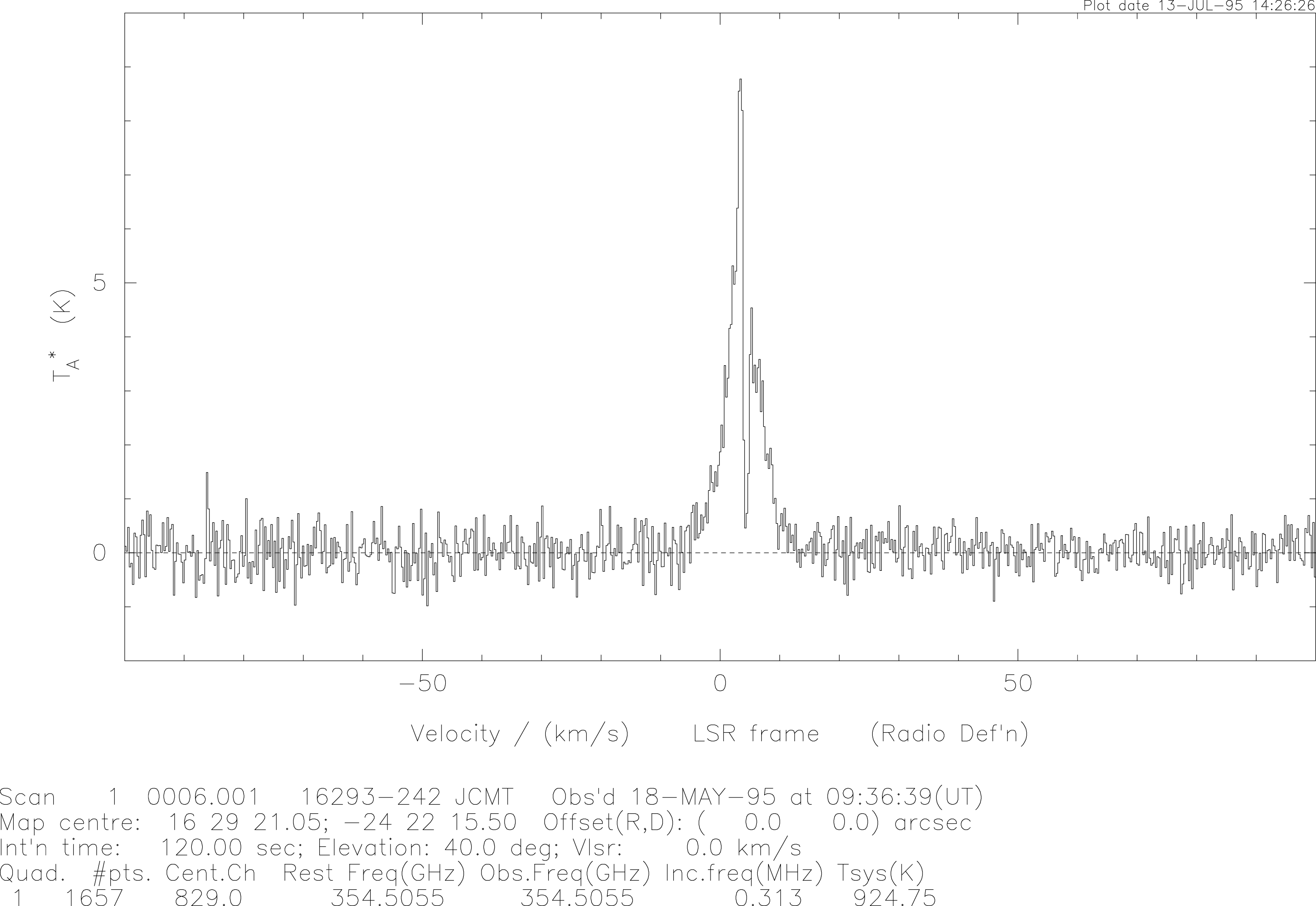
The spectrum can be plotted in two ways: histogram (the default on startup), and line (connect the dots). One can also set the line thickness and the colour (set to 1 and 3 [=green] on startup). The first two are controlled by the flags histogram and line_weight. That is, on startup the defaults are

$>>$ histogram=true
$>>$ line_weight=1

Typing histogram=false gives a line plot. I wouldn’t recommend using a line_weight larger than 3. Colour numbers range from 1 to 15.

3.4.1 Closing in on your spectrum; interactive vs non-interactive modes

If you are in interactive mode, there are quite a few things you can do with the spectrum on the screen. The first thing is zoom in on a small section of it so that you don’t have to look at the parts you can’t explain. There are two ways to do this, both of them easy.

The quick way is to use the mouse cursor (using Xwindows) or the cross-hairs (if you are working with a VTxxx graphics-compatible terminal) to make a box around the part you want to look at more closely. Point the mouse cursor at the position on the Xwindow plot screen, and type a command. If you’re using a VTxxx terminal you use the arrow keys to move the crosshairs around; holding down the Shift key makes the lines move in large steps. Place the cursor position (or intersection of the cross-hairs) on one corner of the box you want to draw and hit one of the following keys to mark the spot; t, b, l, r. For example, to identify the lower right corner of the box you hit b (for ‘bottom’) and r (for ‘right’). Now go to the opposite corner and hit the other two keys (i.e. t for top and l for left). The box will not appear on the screen until you hit d for draw. This will draw the box on the screen. If you made a mistake drawing the box just try again. When you’ve got the box you want hit n for new_limits and the portion of the spectrum inside the box will be replotted. Table 1 (taken from Rachael Padman’s SPECX manual version 6.3) shows other possibilities; I’m sure the options have increased in number since then, so use the h option (for ‘help’) to see a complete list.

If you want exact limits on the axes you can use the second method. First figure out what the x and y limits are from your plot. Lets say, for example that you want the x axis to run from $-50$ to $+50$ km/s and the y axis from $-5$ to 50 Kelvin. You would use the set-plot-scales command:

If you want to see all of the spectrum again then send the following;

Note that you can set either of the x and y scales to automatic scaling, or both. This is a very useful feature.

3.5 A note on command line syntax

This may be a little tedious by now, so this may be a good time to introduce the notion of dispensing with the chatter of the question-and-answer mode. Once you know what questions SPECX will ask you can provide the answers before being asked on a command line. Thus, to set the plot scales above you would type

$>>$ s-p-sc\n\-50 50\n\-5 50\ 

and to reset the scales to fully automatic

$>>$ s-p-sc\y\y\ 

Note that the command itself has been shortened to the minimum-matching level. If you truncate the command too much SPECX will inform you of all the commands meeting your ambiguous specification. The backslashes separate command line parameters. They do not have to be present in this particular case i.e. 

$>>$ s-p-sc y y 

would do. However, it is better to have them there within command files, especially where a command calls for multiple inputs. Otherwise the results may be a little strange on occasion.

Parameters may be omitted altogether if you want to take the defaults, or the previous settings. In this case one can either use the placeholder symbol #:

$>>$ s-p-sc\n\#\n\#\ 

or nothing at all:

$>>$ s-p-sc\\\\\ 

3.6 Dressing Up Your Spectrum

Now that you’ve got your spectrum on the screen you can make it look a little better by doing some simple operations on it.

3.6.1 Smoothing the data

The most common operation is binning over a number of channels. SPECX asks you how wide the bin should be. It averages the points in the bin and plots the average. So if I want to have a bin of width 5 for the current spectrum I would send the following command:

A similar operation is smoothing. SPECX produces a running mean over the spectrum. If I want to smooth the current spectrum using a 5-point average the following command will do it.

or in a shorter version;

$>>$ sm-sp 5 

There are also operations like hann-spectrum, convolve-spectrum, fold-spectrum etc. A comparison of binned and smoothed spectra is shown in Figure 3. Note that the number of channels in the end spectrum is different in each case. For a DAS spectrum having 1657 channels after merging (see later), Hanning-smoothing (hann) reduces that to 1655, running-mean smoothing over 5 channels (sm-sp 5 gives 1653, and binning over 5 channels (bin 5) results in only 331 channels. These differences become very important when making maps. Hanning-smoothing is very effective at removing ‘ringing’ caused by spikes in the data (cf. Section 3.14).

Figure 3: Using various channel-averaging methods. In order, from bottom to top, the spectra are (a) the original, (b) Hanning-smoothed (using hann), (c) smoothed by 5 channels (with sm-sp 5), and (d) binned over 5 channels (using bin 5)

3.6.2 Putting vertical and horizontal lines on the spectrum

There are times you may wish to guide the eye of your readers to some feature of your spectrum. A vertical line (extending the entire height of the spectrum plot frame) can be put at, say, 56 km/s by typing:

$>>$ vert 56

A plot has to be open for this to work. The plot will be redrawn.

In SPECX 6.3 I didn’t find any equivalent for horizontal lines, but if you really want to do this, one method that works is to multiply your spectrum by zero number, offset to where you want it vertically, and replot the spectrum. Thus, say:

$>>$ mult 0.0; off 2.5; over 1 6

would put a horizontal line on your open plot 2.5 K above zero. This also allows one ready control over both line width and color. SPECX 6.7 includes the baseline command which implements this sequence for you.

3.7 Getting To Know Your Baselines

If you want to start a little data reduction on your spectrum you can remove some baselines or fit some models. There seems to be some controversy about the names of the commands though. Some people claim that a gaussian is not a baseline, it’s a model. The difference lies in whether one is removing an instrumental ‘baseline’ or curve which underlies the line itself, or whether one is fitting the line itself with a ‘model’.

When fitting baselines or models, or doing a number of other operations on spectra, one or more sections of the spectrum need to be specified. For a linear baseline fit, two regions of the baseline need to be identified for the fit. In the case of polynomial fits, one to several such regions can be specified. And for a gaussian fit, one specifies not the baseline, but the line region to be fit. It all makes sense really. Just try it.

One can specify the fit regions either in interactive mode, in which case the cursor (or crosshair) is used to define sections of the spectrum, or by specifying the same sections by typing in the numbers in non-interactive mode. In my view interactive mode can be a pain to use, but the results are worth it. The procedures outlined next for fitting a linear baseline will apply to all situations where x-value ranges are called for.

3.7.1 Linear baselines

To take a linear baseline out of your spectrum use the command remove-linear-baseline. For example, I want to remove a linear baseline from the current spectrum. The following command will do it:

$>>$ r-l-b

If you are in interactive mode the screen will display the current spectrum with the first of the previously chosen boxes (if any) outlined in dot-dashed lines. If you are using Xwindows click first on the title bar at the top of the plot window – it will be labelled “PGPLOT Window 1”; depending on how your system is set up clicking elsewhere in the window may give erroneous results. Then either

• tap the return key at this point to choose the range shown (which will then be displayed in solid lines), and display the second range. You have the option of taking this one too, in which case you are finished with this fit.
• or, alternatively, move the cursor or cross-hair to a somewhat flat part of the noise to the left of the spectral line and hit ‘l’ (for ‘left’) and then move a little to the right (still to the left of the spectral line) and hit ‘r’ (for ‘right’) and finally ‘a’ (for ‘accept’). Now a box will appear on the screen corresponding to the range between the chosen l and r positions. Now go to the right side of the spectral line and do the same thing. When you hit ‘a’ this time though, the baseline will have been subtracted and the end result will be in the current spectrum buffer.

To see the end result, all you need to do now is type ‘n’. Remember, to get out of the interactive mode, type ‘e’ with the cursor anywhere inside the plot window. If you want to leave the interactive mode altogther use the command

$>>$ s-i n

In non-interactive mode the following exchange is typical. The result in this particular instance is shown in Figure 4. Remember, EOF is Control-d.

Figure 4: The upper spectrum is the original after averaging several observations. Basically in this case there is an offset in the baselevel due to the continuum background of the source (G34.3). Below it is the effect of removing a linear baseline tied to clean (line-free) regions of the spectrum.

3.7.2 Polynomial baselines

Fitting a polynomial baseline is similar, by using the command

$>>$ fit-polynomial-baseline

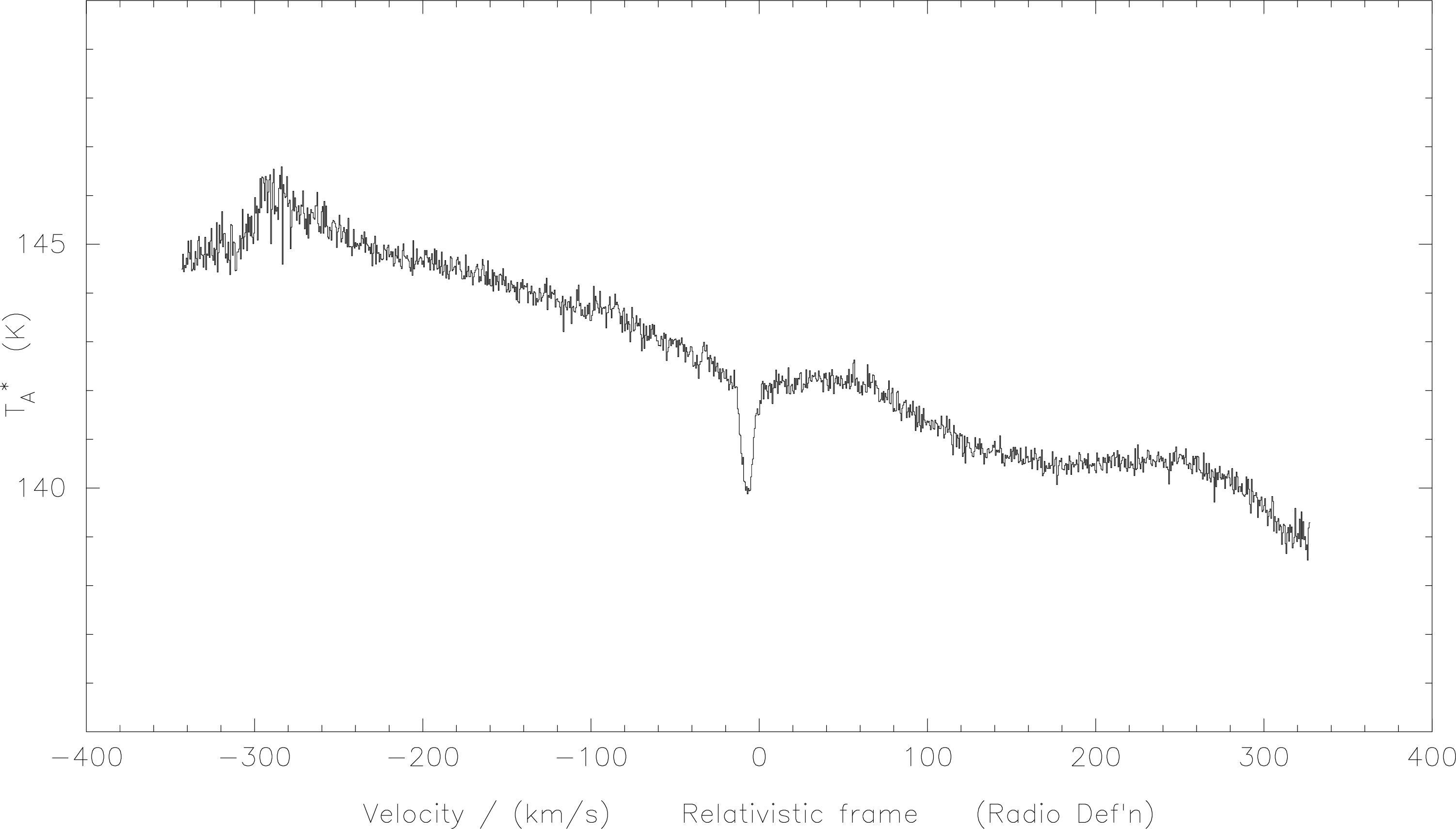
f-p-b will do. A typical bad baseline requiring a polynomial fit is shown below in Figure 5.

Figure 5: This spectrum was obtained towards a bright planet. The penalty is the poor baseline, even though beam-switching in azimuth was used.

Again, in interactive mode the screen will display the current spectrum and you have to tell it where to fit the polynomial. There are two differences from a linear baseline removal though; first, you can choose one or more regions, and second, after you fit a baseline SPECX won’t remove it until you tell it to. You use the same keys as before, l for the left boundary of a region, r for the right and a to accept the region. When you are done marking regions, hit the e for exit and SPECX will ask you for the order of polynomial you want and then make its fit.

In non-interactive mode the exchange might look like:

The fitted baseline is now the current spectrum in the x-register, so if you want to look at it just use the overlay command; e.g.:

$>>$ over 1 5

As shown in Figure 6 this will plot the fitted curve on top of the original spectrum.

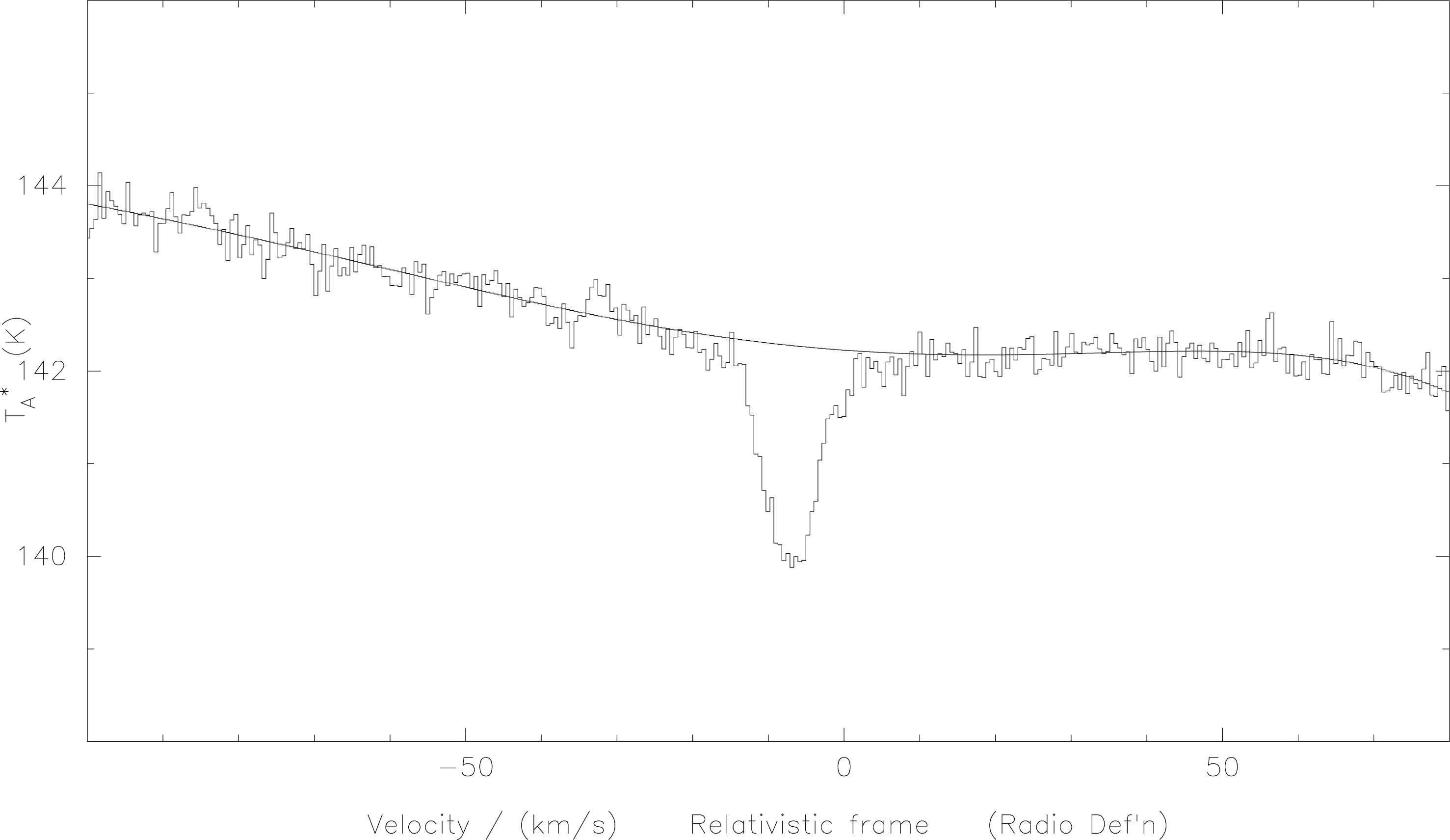
Figure 6: A portion of the baseline of the spectrum in Figure 5 fitted with a polynomial function using f-p-b. The polynomial has been overlaid on the original spectrum.

To remove the baseline from the spectrum you subtract the fit from the original (this places the difference in the top buffer): i.e. to subtract the fit and display the result type

$>>$ sub;n

In the cases of complex baselines in which you see baseline ripple (i.e. sinusoidal effects) using the command fit-composite-baseline (f-c-b) can be a better choice. However, it is necessary to experiment with this command to achieve the best results.

3.7.3 Gaussian models

Gaussian fitting is done in a similar way. The only difference is that here you need to specify the line region, rather than outside it. You will be asked for initial guesses for the amplitude, width and position of each gaussian you want to fit. A helpful hint here is to make use of the ability of SPECX to write output (such as Guassian fit parameters) to a file. To do this type

$>>$ s-l-f f file-name

where file-name is your choice of file to which to write the information. Remember to reset the output to your screen subsequently (use s-l-f t).

The key commands here are fit-gaussian-model and calculate-gaussian-model, f-g-m and c-g-m respectively.

In non-interactive mode, the dialog might proceed as follows:

What happened here was I used f-g-m to fit the velocity range surrounding with two Guassian components as specified. Then I used c-g-m to calculate the curve corresponding to these components (which is placed at the top of the stack) and then plotted it on the same axes as for the spectrum. The result of this is shown in Figure 7.

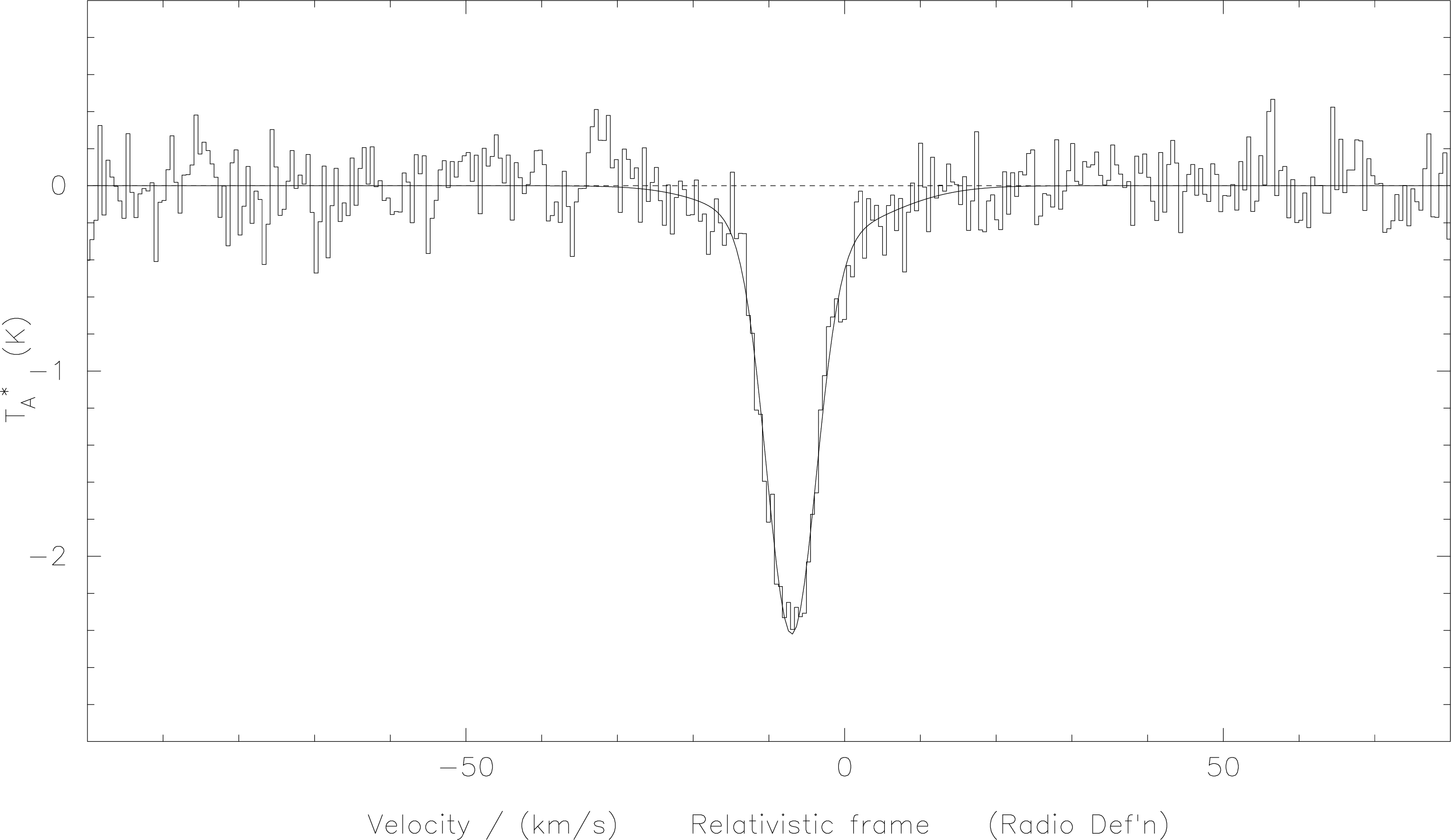
Figure 7: The spectrum in Figure 6 after subtraction of a polynomial baseline, showing a fit, plotted as a continuous line by using histogram=false, of two gaussian components as given in the example in the text. Fitting two gaussians may be a little misleading here, since the broader, weaker component could be a baseline artifact, or could result from pressure broadening of the line. In the latter case a Voigt profile should be a better fit.

3.8 The Stack

We have alluded a couple of times to the presence of internal arrays in which data is stored once in a while. Now is the time to formalize that knowledge. SPECX uses a ‘stack’ to keep spectra in order. The stack is modeled after the Hewlett-Packard calculator reverse Polish logic, which some people seem to have trouble with.

Most of the time all you have to remember is that the current spectrum (the one that gets plotted with the n command) is in the x-register. This may (in the case of f-p-b) be a fitted baseline. If you load one spectrum and then another, the first is pushed down into the y-register, and the second goes into the x-register. The command ave averages the two, and places the result into the x-register. This is all carefully described in the SPECX manual. However, in case you need to understand more (that is, you happen to be a Luddite who likes the typical department-store calculator better than an HP), you can see the contents of the stack using the command

$>>$ show-stack

For department-store calculator people it’s important to know that the stack is upside-down. Position X is the bottom and T is the top. The spectrum in the bottom register is the current one.

There are four operations you can do to move the stack registers around and one command to clear the stack which is, of course, clear-stack. The four operations are; xy-interchange, roll-stack, push-stack-up, and pop-stack-down. xy, roll, push and pop will suffice.

Table 2 shows the results of these four commands.

3.9 Saving Reduced Data for later

3.9.1 Using Data Files

As you can see, the stack is not a good place to keep a spectrum after you have spent time removing baselines and smoothing it. It can easily get lost in the shuffle of the stack. The safe place to keep a polished spectrum is in its own special file which you can close and re-open later when you have time.

A single file can contain any number of spectra. First you have to open a file with the open-file command. Then SPECX will ask you what you want to call the file, and a couple of other questions.

Lets say I have just removed a baseline from my spectrum and now I want to save it for later. For now I only want the one spectrum in the file, but I can put more in the file later; the file is in principle infinitely expandable. The name of the file will be stanley (under Unix the file will be called stanley.sdf; the filetype .sdf is the default). Here is the command dialog:

The answers to the questions about file title and owner are not crucial. They will only appear if you make a listing of the file contents. However, do not allow spaces, dashes, or semicolons to appear in either field, or, for that matter, in the filename; otherwise the results will not be what you wanted.

Now a file stanley.sdf will appear in my directory. To get the data into the file you use write-spectrum. This puts the spectrum in the stack X register into the file. So I do the following command;

When first created the file access is set to write-only. When opened on subsequent occasions the default file access is read-only. If you want to change this use the set-file-access command:

To close a file use close-file. You can have up to eight files open at any one time. If you want to see which files are open, and what their access rights are, do;

To retrieve a spectrum from a file you use the command read-spectrum. The file you want to read has to be open and have read access: e.g.

3.9.2 Temporary Storage

Several storage registers are available to allow intermediate results, such as a partial average, to be stored temporarily. To store the contents of the stack X-register in storage register 2, type:

$>>$ sto-sp 2

To retrieve it at a later time, type:

$>>$ reca-sp 2

3.10 Using das-merge

For observations using the DAS it is necessary to remember that for all but the narrowest bandwidth (125 MHz) the spectrum obtained consists of 2, 4, or 8 subbands. As noted elsewhere, these subbands are contiguous in channel space, but overlap in frequency/velocity space. Each subband has edge effects which should be removed before gluing the spectrum together. The function das-merge uses a specified number of overlap channels from the ends of each subband to average the overlap regions, optionally with vertical realignment of the subbands.

3.10.1 The Principles

If one were to plot a spectrum before using das-merge one would obtain something like the spectrum in Figure 8.

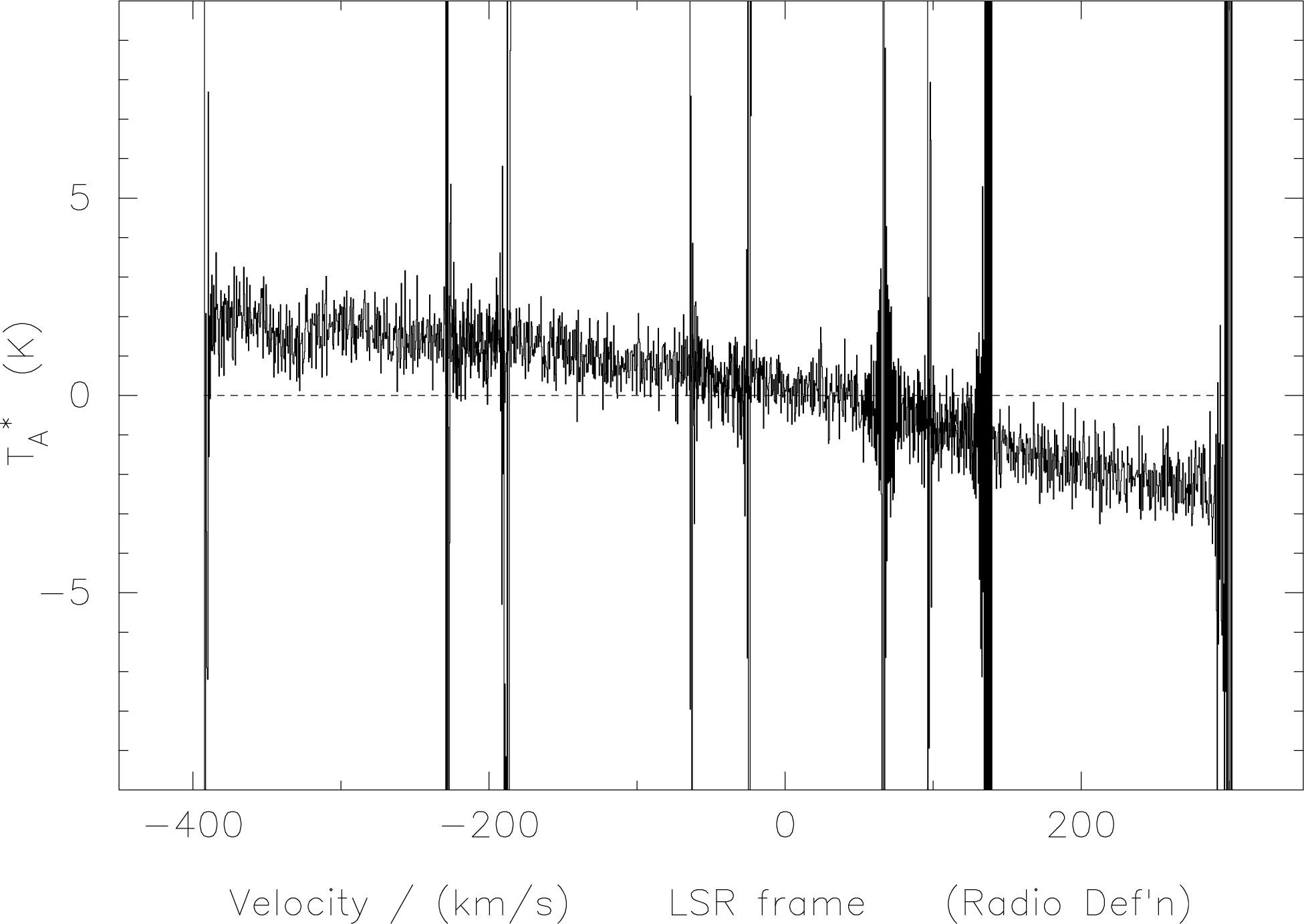
Figure 8: A spectrum consisting of 4 subbands (500 MHz total bandwidth) taken with a very short integration with receiver A2, plotted without applying das-merge. The edge effects of the overlapping subbands appear as sharp spikes; one spike, at 70 km/s is however due to interference within the bandpass.

For illustration purposes, if we stagger the subbands vertically using the set-quadrant-display and offset commands in tandem, then the overlap between subbands becomes clear, as in Fig. 9.

Figure 9: The spectrum before applying das-merge. Quadrants are offset from each other for clarity.

das-merge in fact combines two commands. First it strips off the spiky ends of each subband, using the drop-channels command. The best number of channels dropped from each end of each subband depends on the bandwidth to some extent, but is typically 15–30. The default is set to half the subband overlap. Using the same staggered subband display for clarity the end result looks like that in Fig. 10.

Figure 10: The spectrum after applying das-merge. Quadrants offset from one another for clarity.

Note that the subbands still have significant overlap in velocity space. This overlap is used to facilitate the second part of the das-merge action, which averages signals in the overlap region. This can be done separately using the merge-quadrants command. The end result in this instance is shown in Figure 11.

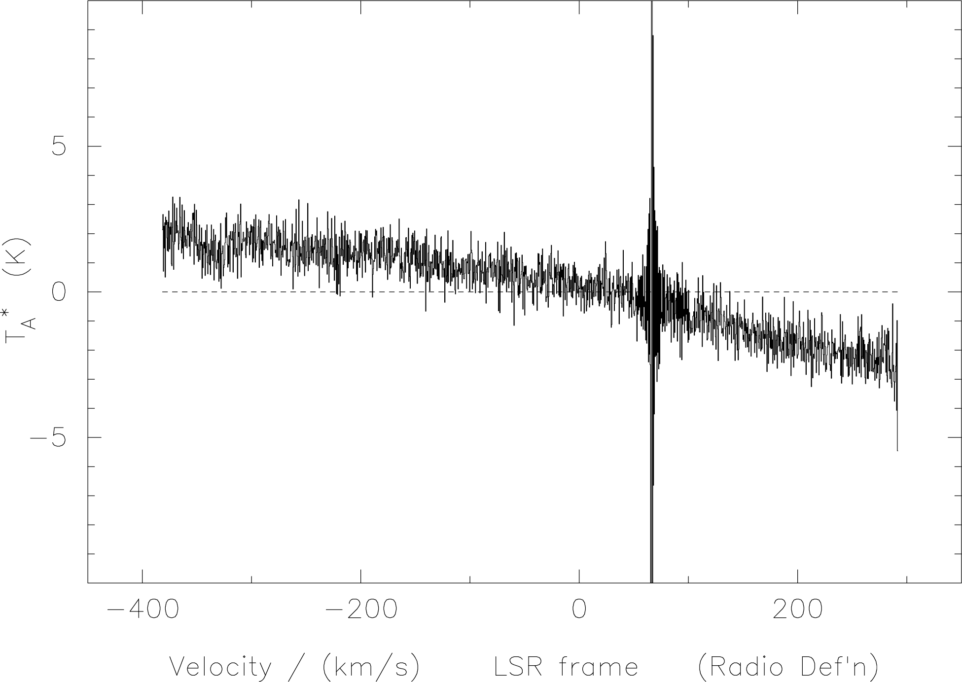
Figure 11: The spectrum in Figure 8 after application of das-merge. The subbands are successful merged into a continuous spectrum. Only the interference spike remains.

Note that if one has previously modified the effective rest frequency using the s-l-r-f command (see Section 3.16.2) then one must reset the rest frequency to accept the default header values associated with the next spectrum before das-merge can be used. That is, one must issue the command

$>>$ s-l-r-f 0.0

first. The consequence of not doing this is that the first subband of the new spectrum appears to das-merge to not have the correct frequency, and the error message

will result. This is your clue to the above common problem, if you are given to mess with the frequencies.

3.10.2 Caveats

The defaults for das-merge work well for most purposes; that is, taking the default number of channels for removal, then refusing the vertical adjustment between subbands. Long integrations suggest that it is correct not to take the vertical subband adjustment. The intrinsic flatness of the DAS response is excellent, and applying the subband adjustment actually can introduce low-level offsets between subbands, which, particularly for wide weak lines, could result in spurious detections. Hence one should use the default command, equivalent to

$>>$ das-merge$\setminus$#$\setminus$n$\setminus$

for almost all cases.

One particular case which can readily introduce baselevel offsets if one applies the vertical subband adjustment is when one has a bright line in the central overlap region. One such example is shown in Figure 12. In such case one should most definitely use the default ‘n’ option.

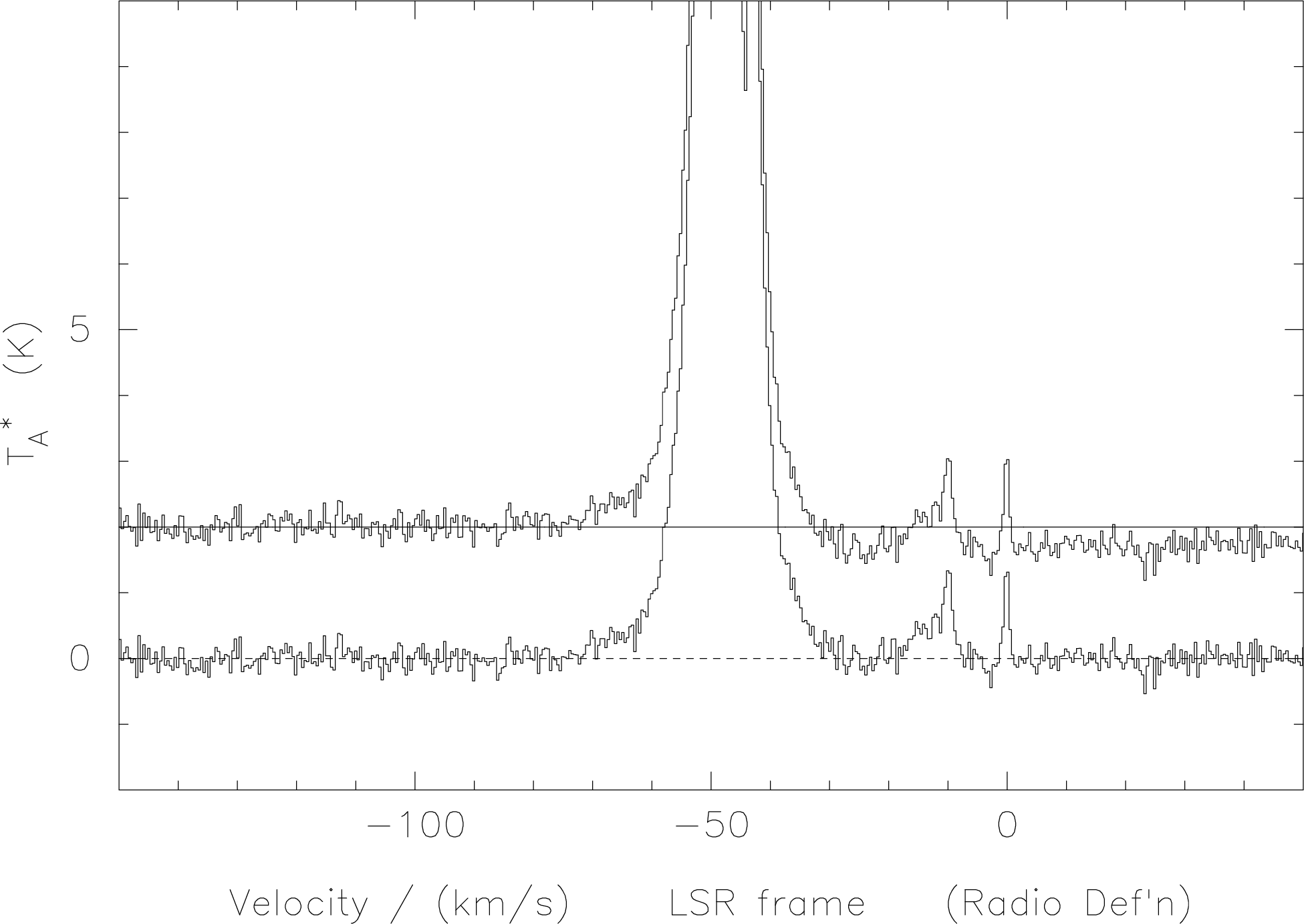
Figure 12: The same CO(3–2) spectrum of W3(OH), reduced using das-merge with subband offsets (upper spectrum) and without (lower spectrum). The presence of the strong line in the overlap region introduces an artificial baseline step in the former instance. One should use das-merge$\setminus$#$\setminus$n$\setminus$ here for sure.

Possibly the only time the ‘n’ option may introduce artificial effects is when observing a planet. Even then the effect is likely to be small. See Figure 13.

Figure 13: The upper spectrum is an observation of Saturn using the 8-subband 760-MHz mode with B3i; the result is normalized to an observed value of 90 K T${}_a^{\ast }$ (i.e. the actual value is about 45 K), and subband offsets have been applied in this case when using das-merge. The lower curve shows the difference introduced when not using the subband offsets, as compared with the upper spectrum. Using das-merge$\setminus$#$\setminus$n$\setminus$ here introduces additional small steps corresponding to a maximum of about 1% of the total signal.

3.11 Dealing With Multiple Spectra

3.11.1 Averaging Several Spectra

SPECX is able to average only two spectra at a time. If you want to average several spectra you will have to do a little juggling with the stack.

For example, if I want to average spectra 1 through 5, I would have to do the following. Read in spectrum 1, read in spectrum 2, average them, read spectrum 3, average again, read spectrum 4, average, read 5 and average one more time.

Thus to average five spectra (131, 132, 133, 134 and 135, say) you would type:

$>>$ r-g-d 131
$>>$ r-g-d 132; ave
$>>$ r-g-d 133; ave
$>>$ r-g-d 134; ave
$>>$ r-g-d 135; ave

Generally, if you have learned to put all the necessary commands on one line you can repeat the sequence of using the ‘up-arrow’ key and editing the line. If you have to do it very often, it would probably be smart to write a command file (see Section 3.15) or an in-line do-loop (see Section 3.15.4) to do it for you. Such a do-loop might go like this:

This would then average your spectra. Certainly less typing if you have a lot of spectra in sequence(s) to average. Note that having done the do-loop once creates a file called temp.spx which does the same thing as the do-loop we just made. So if you had two more groups of spectra (say, 138–143 and 145–150) to average with the preceding average, just type

$>>$ @temp 138 143
$>>$ @temp 145 150

to complete the set of spectra to be averaged.

3.11.2 Displaying More Than One Spectrum

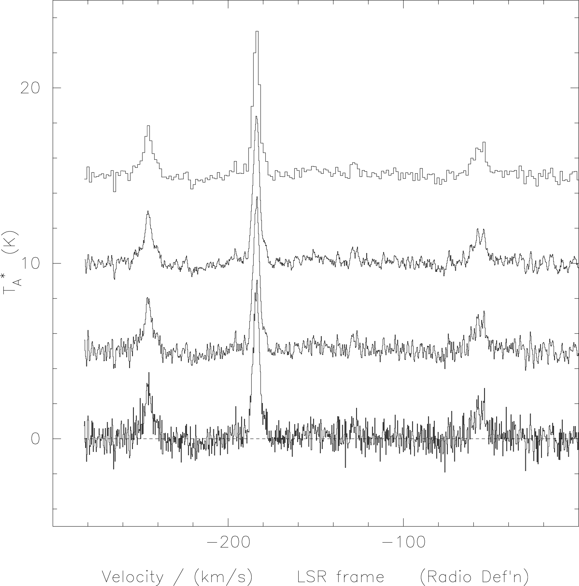
In Section 3.6 there are some plots with more than one spectra. The ability to plot two or more spectra on one set of axes is very useful sometimes.

When you send the new-plot command SPECX closes the old plot file and opens a new, clean one. The trick of getting more than one spectra is not to close the plot before you’re done adding things to it. This is done using the overlay command, as we have already seen. There is a close-plot command by the way, which is useful particularly when you are working with output to a plotfile ultimately destined for printing.

You can keep on using overlay for any number of spectra. If you want a decent plot remember to offset them vertically one from another (use the offset command). Also, you can’t change the plot scales after you’ve opened a plot so make it big enough before you start.

3.12 Concatenation – combining spectra lengthwise

If you have several independent spectra for which the velocity/frequency ranges are cover a wider range than any one such spectrum, it may be useful to combine them on a single plot. This is a trivial application, since all one has to do is increase the length of the x-axis of the final plot sufficiently to allow yourself room to plot all the spectra using new-plot and successive applications of overlay. There are however, a couple of more specialised applications, which we get to next.

3.12.1 Making very long spectra

There is a much less trivial application than the above which occurs when one has spectra which occupy both subsystems of the DAS. Consider a CO 4-3 observation with receiver C2 in the special wideband mode; in this case there are 16 subbands, using both subsystems, and extending over nearly 1.8 GHz. Each subsystem consists of eight subsections. Loading this spectrum into SPECX shows that two positions in the stack are used, one for each subsystem:

The following sequence of commands will reduce this to a single spectrum (dialogue has been omitted):

Here one first performs the das-merge on each of the subsystems separately, then concatenates the two spectra to produce a single version which has overlapping channels around the centre, and finally merges both spectra together to form the final result. Normally the comamnd merge-quadrants is used only as part of das-merge, but it can be used separately, as in this instance.

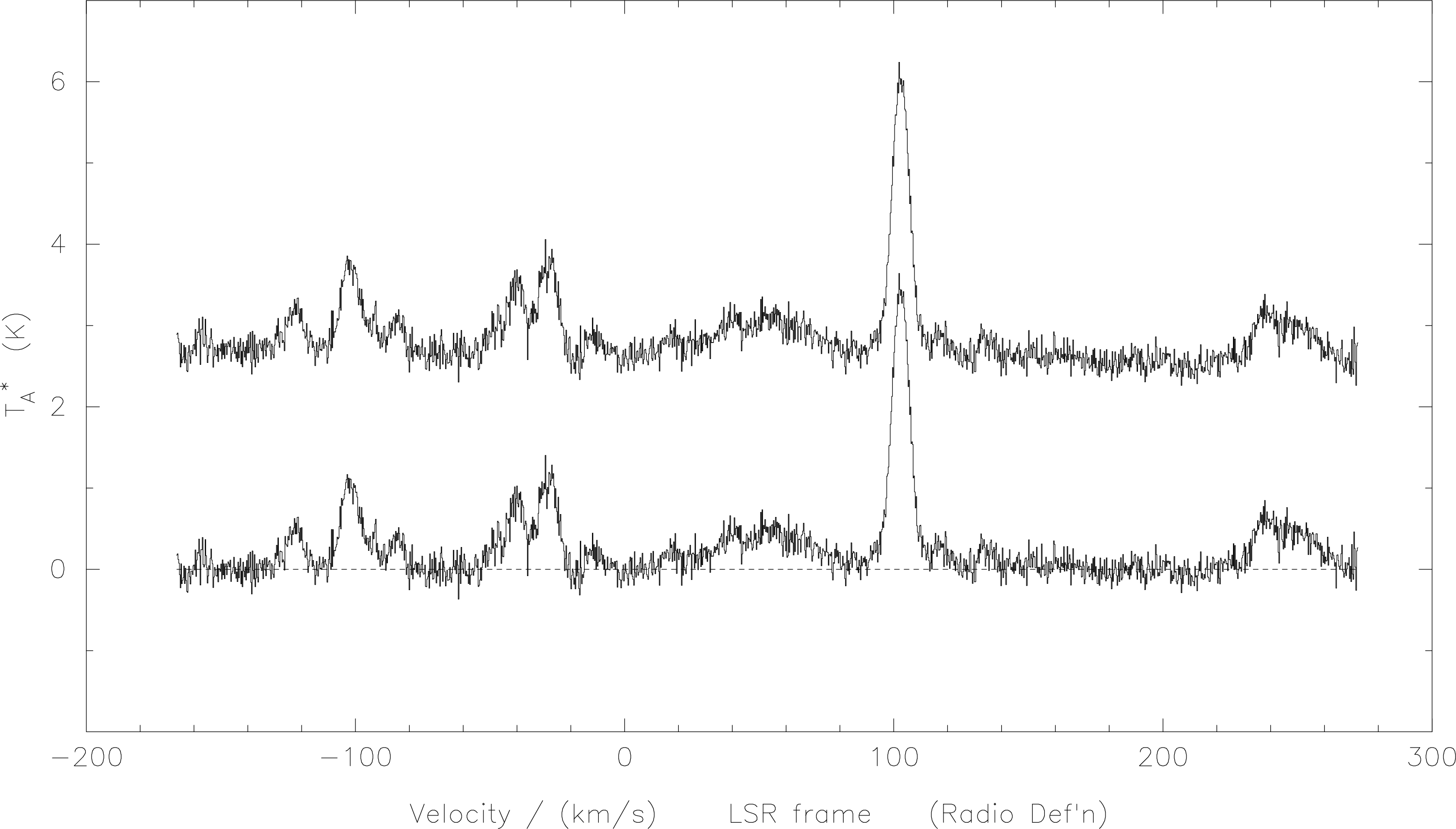
Doing this to the next spectrum, averaging the result, and so on for all the spectra in a set one can form the final average (see Figure 14). It would make sense to construct a procedure to do this (see later).

Figure 14: An example of a spectrum taken in the dual subsystem mode with receiver C2, covering about 1.8 GHz, after concatenating and merging the two subsystems.

3.12.2 The special case of the 750-MHz mode

The 750-MHz mode of the DAS was used for a short time only for receiver A2, and is no longer in use. In this case there were two subsystems of 4 subbands each. A similar approach can be taken in this case, to that used for the ultra-wideband mode discussed above.

3.13 Arithmetic With Spectra

As you saw before when I was removing baselines, you can subtract the X register from the Y register and have the difference become the new X register. The command is subtract-spectrum. SPECX can also add the X and Y together and average them. The commands are add-spectrum and average-spectrum. average-spectrum (ave is enough) is the usual choice, and uses weights when averaging that are determined by the integration time divided by the square root of the system temperatures of the two spectra.

While I’m on the subject, SPECX also has multiply-spectrum and divide-spectrum. Skipping the conversational mode the commands would be e.g.:

$>>$ mult 2.0

and

$>>$ div 7.8

The defaults factors are set to unity (they used to be zero).

3.13.1 Spectrum Statistics

At some point during your data reduction you might want to know a little more about your spectrum. There are several commands which determine the parameters of spectra. Two of the more useful commands are find-spectrum-statistics and find-integrated-intensity. There are others in R. Padman’s manual.

To use these commands in interactive mode you get a plot of the current spectrum like you did when removing and fitting baselines so that you can specify a region. Just use the cursor or crosshairs and l, r, and a as you did before.

Once again it may be useful to write the outputs to a separate file using the s-l-f command.

3.14 Dealing with spikes

External (or internal) interference (RFI) is a common occurrence with the longer wavelengths in use at the JCMT; that is, particularly in spectra taken with receiver A2. Usually this is offset from the centre of the band and is of no major concern. It seems to be worse for position-switching and may disappear entirely in the azimuth beamswitched mode. Sometimes, however it can be a real nuisance. An example is given in Figure 15.

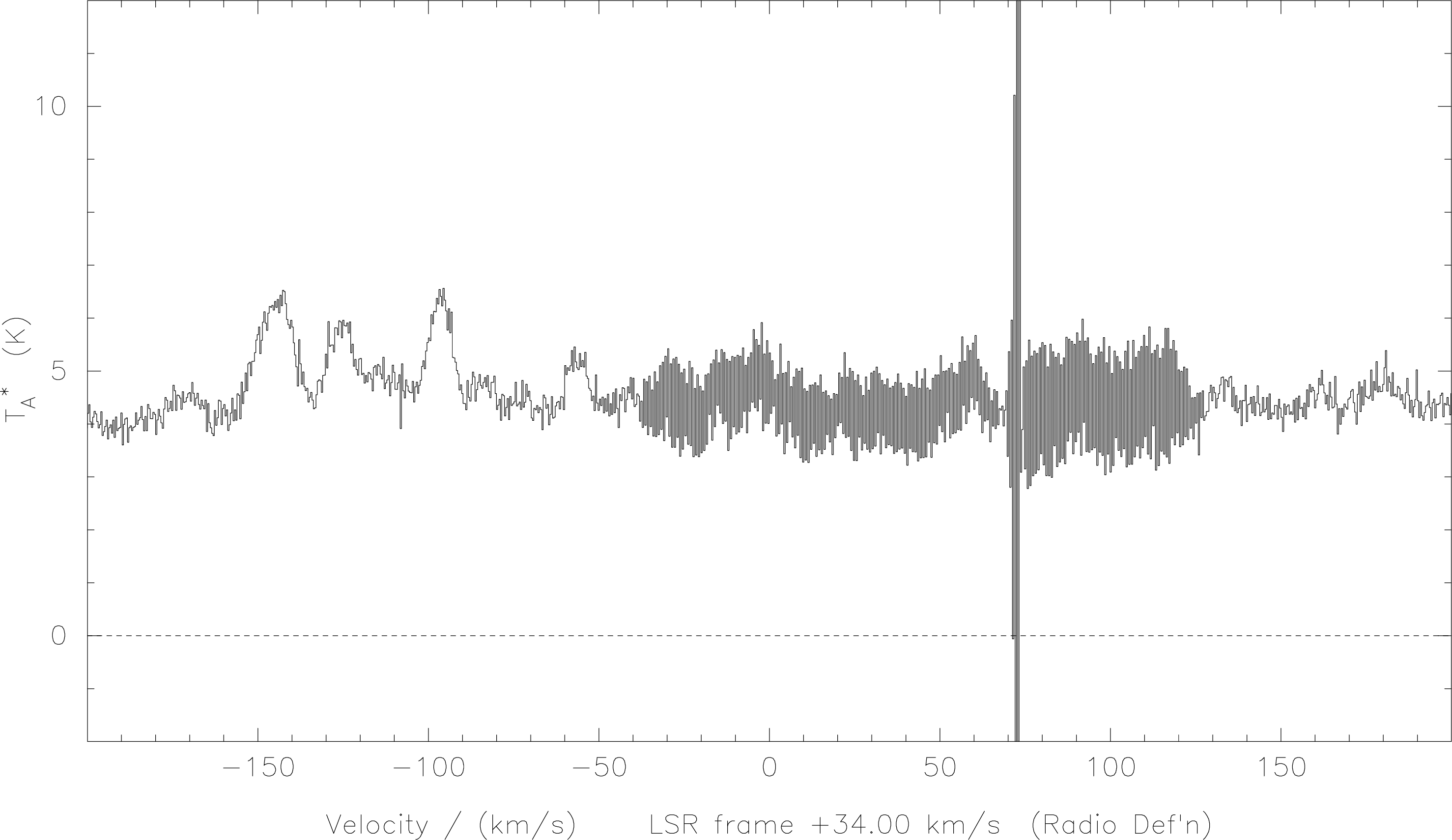
Figure 15: A position-switched DAS spectrum of G34.3 in the area of 239 GHz showing ‘ringing’ caused by a strong internal interference spike. Note that it affects only the subband in which it occurs. The offset from zero is the result of a combination of the source continuum emission and a difference in the airmass between the signal and reference positions. The line features are due to CH${}_3$CCH and CH${}_3$CN.

Such interference spikes may be very effectively removed by applying Hanning smoothing to the spectrum:

$>>$ hann

The result is shown in Figure 16. A multitude of weak line features, as expected, are now revealed. The spike itself may be removed by using the spike-removal command:

$>>$ rem-spike

Figure 16: The result of applying Hanning smoothing to the spectrum shown in Figure 15. Note that the ‘ringing’ completely disappears, revealing previously obscured line features. The spectrum is itself somewhat smoothed in the process.

3.15 Writing Your Own Command Files

To save time and keystrokes when reducing your data, you can write command files that will do the tedious work for you. When writing command files it is usually faster to be outside of SPECX. To do this you can either do

(1)

$>>$ exit; which will take you out of SPECX completely, or

(2)

$>>$ $
Shell command line?

This is your cue to enter any shell command that you would like, such as, say,

  emacs &

to start up emacs in a separate window which will remain until you specifically close it.

(3)

You can just type this without asking for the prompt, of course:

$>>$ $ emacs &

(4)

If you are using a windowed terminal, open a completely separate xterm, say, for the purpose.

A command file is very simple to understand because it’s just a list of SPECX commands. The only pitfalls are knowing what order to submit the commands to SPECX and knowing in advance what questions SPECX is going to ask. This implies a little experience is useful before trying to write your own command procedures. Which is why this information is not placed earlier in this Cookbook.

3.15.1 The Basics

Here’s a simple example of a command file. I want SPECX to read observation number 137, das-merge it, smooth the data over a 5 point average, and plot it. First, here are the commands that one would give in SPECX:

$>>$ r-g-d 137
$>>$ das-merge\\n\ 
$>>$ sm-sp 5
$>>$ n

These lines would be faithfully reproduced in a command procedure. You would type, say:

in a separate xterm window and you will be in the pico editor. The latter is simple because there are rather few commands and the basic ones are always displayed at the bottom of the editing window. If you have an aversion to the complexity of emacs this may be the one to use. Now just type the same one line entries as you would inside SPECX. When you are done type Control-o and you will be prompted for the file name you want to write out (a.spx, say, remembering that all SPECX command files are of filetype .spx) Now the file a.spx has been created. To use it, I get back into SPECX either by clicking back on your SPECX window.

Then, back inside SPECX type

The @ tells SPECX to start running a command file. Notice you do not use the suffix .spx in the command.

This was a very silly command file so let’s write one that is a little more useful.

3.15.2 Repetitive Operations

You will recall that when you want to remove a linear baseline from a spectrum or do a similar operation, you had to tell SPECX what region(s) to use from the spectrum. This would hinder automatic operations severely since you would have to sit at the terminal and use the cursor to tell SPECX what regions to use. The way out of this is to always use non-interactive mode:

Now SPECX can carry out things like remove-linear-baselines without plotting the spectra on the screen, and asking lots of questions first. The advantage is when you want to use the same regions for removing baselines, or a similar operation like find-spectrum-statistics in several spectra. For instance, I want to use the regions from $-40$ to $-20$ km/s and from 20 to 40km/s for removing a linear baseline from several spectra, put them into a file called gooddata.sdf and have it repeat the command until I’m done. I would write the following command file, which I’ll call rlb.spx:

The ? in the first line will prompt me for a scan number every time I run the command file. I have specified the linear baseline fit regions between the backslashes, which indicate where responses are be expected to anticipated questions from the SPECX command. I put the data in file number 1 with the wr-sp command, which is gooddata.sdf (I’m assuming you had no other open files). To run the command file type

$>>$ @rlb

and SPECX will ask which scan you want to read (because of the ?). Alternatively, you could type, say,

$>>$ @rlb 137

and the file will process scan 137, without any further ado.

3.15.3 Automatic Repetitive Operations

In the example above, say I want to make a list of the scans to be read in so that I can change the list when I want and go out for doughnuts while SPECX does all the work. One could combine a number of calls to the command file rlb.spx in a simple-minded way in a new command file e.g. 

⋮

Saving this command with some name (say, 1to20.spx) and running it by typing

$>>$ @1to20

processes each of the scans 101 through 120, placing the results in my output file. SPECX will start running 1to20.spx; the first command it gets is to run rlb.spx, and while running rlb it sees the ? and looks for a value, it finds the value in 1to20.spx and continues to run happily along until it gets to the end of 1to20.spx.

This is still a bit silly. Since SPECX allows the use of loops and counters, one can achieve the same result a lot more elegantly. That is, if one creates a command file (call it, say, doit.spx):

then typing

$>>$ @doit

will achieve the same result. The counter n will step from 101 to 120.

As you might guess doit.spx could look like this also:

Taking this still one step further allows the input of parameters from outside:

In this case running this procedure will prompt you for the first and last scans to be processed by rlb.spx. Note that (a) the declaration of the type of variable (I4) required by SPECX for input, and (b) the use of the ask command. The latter gives a prompt (e.g. First scan?) and puts your answer in e.g. the variable fscan.

3.15.4 In-line do-loops

A useful variant of command procedures is an in-line do loop; that is, a set of repetitive operations performed once only without making a command file. To make such a file one begins with a simple do loop statement. Then one is prompted to type in commands, ending with Control-d(EOF). For example, say I want to move a sequence of spectra from a map file and write then to an open file. I might do it this way:

Using the variable i as a simple counter, I read the series of spectra from the map and write then to file number 1. Because there are already spectra in this file, the scan numbers increment from the previous last number.

I mentioned that the in-line do loop is used only once. However, that’s not necessarily true. Such a command file leaves a record of itself in a file called temp.spx. Naturally Unix overwrites this file every time a new version is created, so if you wanted to keep such a file you would have to rename it. The version of temp.spx created by the preceding simple do loop looks like:

This routine could be re-used by simply typing

$>>$ @temp

In-line do-loops are really quite useful. It’s up to your imagination what you use them for.

3.16 Modifying the Velocity and Frequency Axes

There are occasions when it is helpful to change the x-axis on a spectrum. This is particularly true for observations made with offset frequencies designed to accommodate two or more spectral lines from the same or different sidebands. There are four commands which are very useful in this respect:

(1)

set-x enables one to change the x-axis scale;

(2)

with set-line-rest-frequency it is possible to modify the plot so that the spectrum appears as if this frequency had been chosen as the rest frequency

(3)

set-velocity-frame lets one enter a velocity to which the spectrum will be referred in subsequent plots;

(4)

change-sideband shows the spectrum as if it were referred to the other sideband. Use of this command frees the x axis plot scale; to return it to the original setting you will have to undo this effect with s-p-sc.

The effects of these commands tend to cause confusion sometimes, so it may be useful to discuss them a little more. The last three can best be discussed together. One important thing to realise is that the header values of the spectrum are not changed by any of these commands, just the relative positioning of the spectrum in velocity/frequency space for the purpose of plotting. Some parameters, but not all, are carried over into the headers of stored reduced spectra and map files.

3.16.1 set-x

SPECX’s default state on startup is to make all spectrum plots with the x-axis as velocity. This may not always be what you want for clarity, and the command set-x is provided to enable one to plot with a different x-axis. There are three main choices: points, frequency, and velocity. The ‘points’ option is useful for determining which channels to lose from the spectrum if you are planning to make a map.

For instance, the spectrum below (Fig. 17) is typical of those obtained toward OMC-1. Within the band are two lines in which I happened to be interested at the time, neither of which will appear at the expected velocity, because the observing frequency was chosen to allow both lines to appear in the band, and a non-standard DAS mode was used for the observation.

Figure 17: The result of observing with an offset frequency in a line-rich source.

The two lines (of HDO) are at about $-50$ and $-145$ km/s respectively, but it is rather messy to work this out at altitude. It is actually more useful to work in frequency in this case. So, to change from velocity scale to a frequency scale, use set-x and the following exchange occurs:

Note that there is more to this command than just choosing an x-axis. One must also choose the origin, effectively, in this case via the absolute/relative frequency switch. If I had chosen ‘relative’ I would have been asked “relative to what?”.

In this example I chose to turn off the polynomial frequency correction; having this on is useful only for non-linear scales such as that produced by the AOSC. The DAS scale is quite linear by definition. The use of absolute frequency scales enables me easily to see what frequencies my lines have. As shown below in Fig. 18, this provides both upper and lower sideband frequency scales, on the bottom and top x axes respectively. However, these scales will be correct only if one puts in the correct peculiar velocity for your source; otherwise a velocity of 0 km/s is assumed. Thus if the lines have an appreciable peculiar velocity they will appear to have the incorrect frequency. The velocity is specified by using s-v-f. This therefore brings us to the next section.

3.16.2 s-l-r-f, s-v-f and ch-sid

So, if I put the correct velocity in place using s-v-f:

and then changing the x-axis to frequency using set-x we get the result following in Fig. 18:

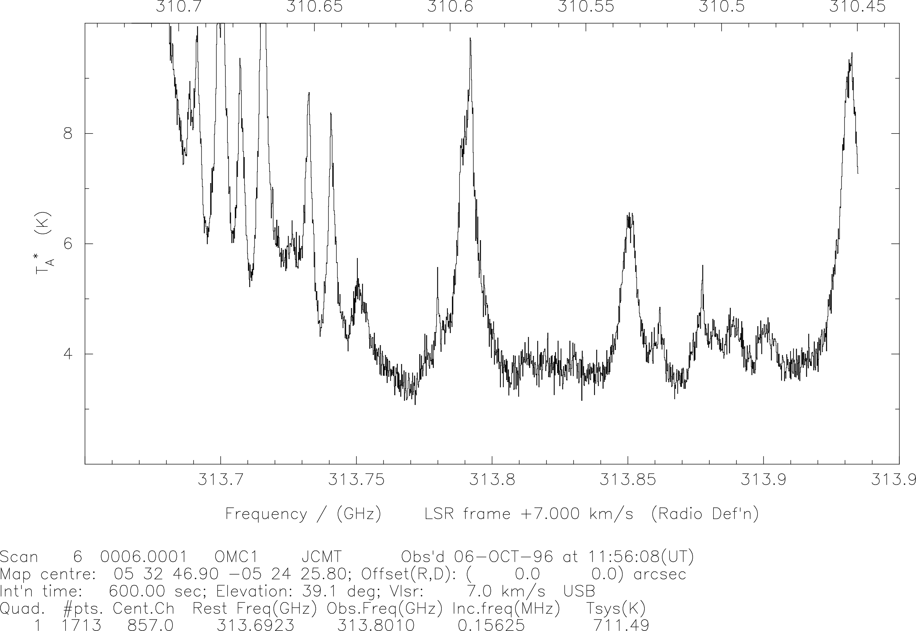
Figure 18: Figure 17 after changing to a frequency x-axis and providing SPECX with the correct lsr velocity.

From these data the two HDO lines at 310.5333 (upper x axis; lower sideband) and 313.7506 GHz (lower x axis; upper sideband) are clearly seen to be present. Of course, the spectrum is reversed now because of the change in axis coordinate, but it makes line identification a lot easier. A subsequent observation at a shifted velocity confirmed this result on this occasion.

Just to show that this all works as expected, we can use a combination of setting the correct line rest frequency (with s-l-r-f) and adopting the other sideband (using ch-sid as appropriate) to display the two lines of interest to good advantage. In this I anticipate the questions SPECX will ask. Then for the line in the upper sideband at 313.7506 GHz:

Note the warning SPECX issues, to let you know that you have modified the frequency/velocity scale. If you want to revert to the default settings you need to type s-l-r-f 0.0. Taking a narrower velocity range the plot looks like that in Fig. 19:

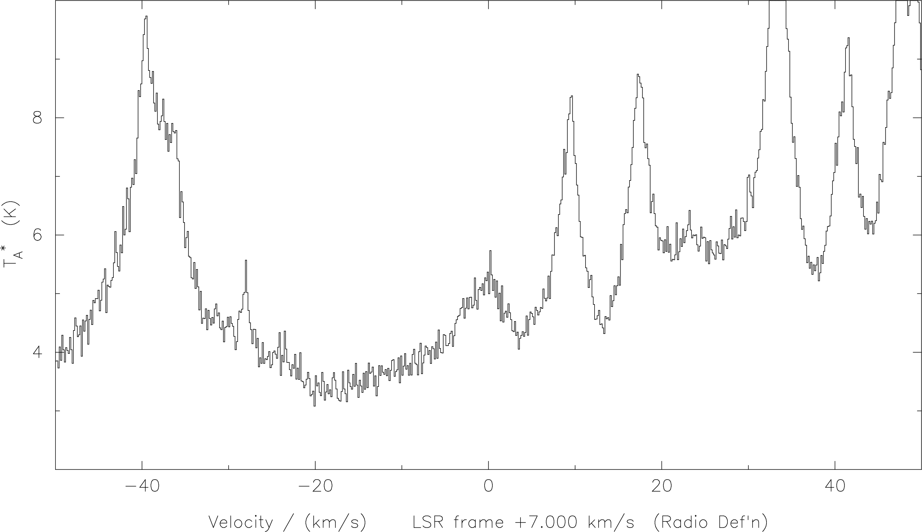
Figure 19: Figure 17 after changing to a frequency x-axis and providing SPECX with the correct lsr velocity, and frequency in the upper sideband.

Here we see that our line is centered at about 0 km/s, because we have referred the scale to an LSR velocity of 7 km/s, the actual velocity of this source.

Once again, note that although the correct LSR velocity was chosen when the observations were made, as seen in the ‘header’ below the plot, this is largely irrelevant to this discussion. We can choose to concentrate on any line by a correct choice of rest frequency, sideband and velocity.

For an equivalent display of the lower sideband line we need to change the sideband also:

Note that ch-sid turns on the default x-axis scaling, and we have to reset this. Then we get the plot in Fig. 20, containing the other HDO line, again centered around 0 km/s:

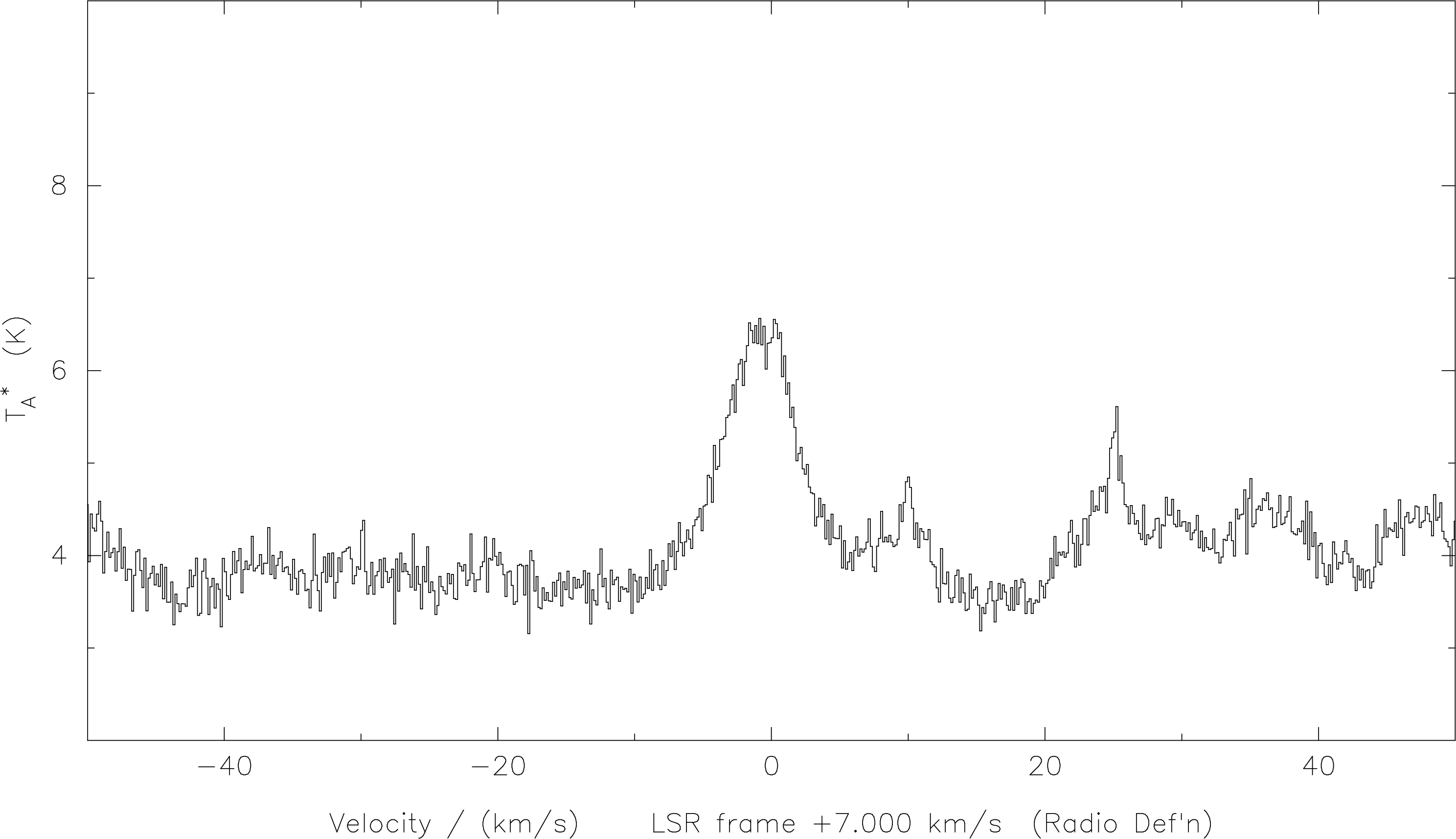
Figure 20: Figure 17 after changing to a frequency x-axis and providing SPECX with the correct lsr velocity, and the frequency in the lower sideband.

Sometimes, because it’s fairly difficult to get everything the way one might want it, it can be useful to collect the commands together in a procedure, which can be edited and re-run until you get the result you want. For example, the following procedure plot three lines which happen to appear in the same spectrum on a common velocity axis. Two of the lines are in the lower sideband, and one in the upper sideband.⁸

The result of this procedure is shown in Figure 21.

Figure 21: Bottom through top: lines of HNC (4–3; 362.3603 GHz), H${}_2$CO (5${}_{05}$–4${}_{04}$; 362.7359 GHz) and H${}_2$CO (5${}_{23}$–4${}_{22}$; 365.3634 GHz) observed toward NGC2071IR; all three lines appear in the same spectrum by virtue of the choice of receiver tuning frequency and IF. The first two lines are in the lower sideband, and the third line comes from the upper sideband. The latter is a fairly high-excitation line (57 cm${}^{-1}$) and thus is quite weak. 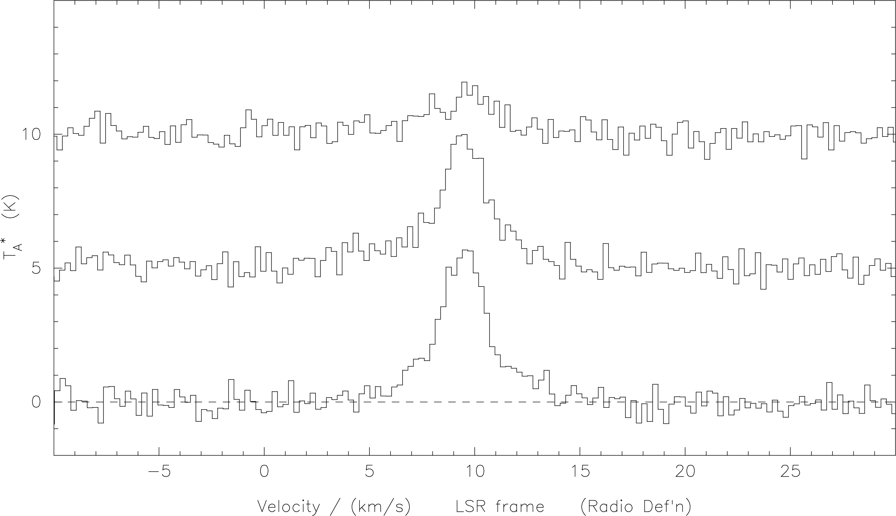Using a combination of s-l-r-f and ch-sid as shown in the text it is possible to plot all three lines on a common velocity scale.

3.17 Reduction of frequency-switched data

For observations taken in frequency-switched mode, the ‘raw’ spectrum consists of two copies of the line profile displaced in both plus and minus frequency directions from the nominal line position by an amount equal to the frequency switch employed. This situation is shown in the top part (‘original’) of the schematic below. Here the nominal line position (at the centre of the spectrometer window) is indicated by ‘+’ and the frequency switch offset by ‘fsw’. There is a positive offset in the signal phase, and a negative one in the reference phase. The spectrum thus has both positive- and negative-going features (‘+L’ and ‘-L’ respectively) corresponding to the two phases.

The data reduction of such a spectrum is done by ‘shifting and adding’: copies of the spectrum are shifted in frequency by plus and minus the frequency-switch amount, and then subtracted. The result is divided by 2 to form the end result, as shown below schematically in Fig. 22.

Figure 22: Schematic – how frequency-switched data is reduced

The final spectrum consists of the line at the correct frequency (and velocity) and two half-height negative ‘ghost’ images of the line (at ‘G’ in the plots above). The separation of the ghosts from the line is $\pm 2.0\Delta \nu$, where $\Delta \nu$ is the original frequency-switch. Any offset and/or slope in the spectrum is automatically removed by this step, but curved baselines are not. A ‘real-life’ example of the above process is shown in Figure 23.

Figure 23: A portion of the ‘raw’ frequency-switched spectrum of the CO(2–1) emission towards L1498 appears at the bottom of this panel. A linear baseline was subtracted for clarity. At the top is the ‘shifted and subtracted’ spectrum. The final CO line profile is at the middle (V$\sim 8$ km/s), flanked by negative-going ‘ghost’ images. The left-hand one of the latter coincides with a ‘ghost’ image from telluric CO, off the frame to the left.

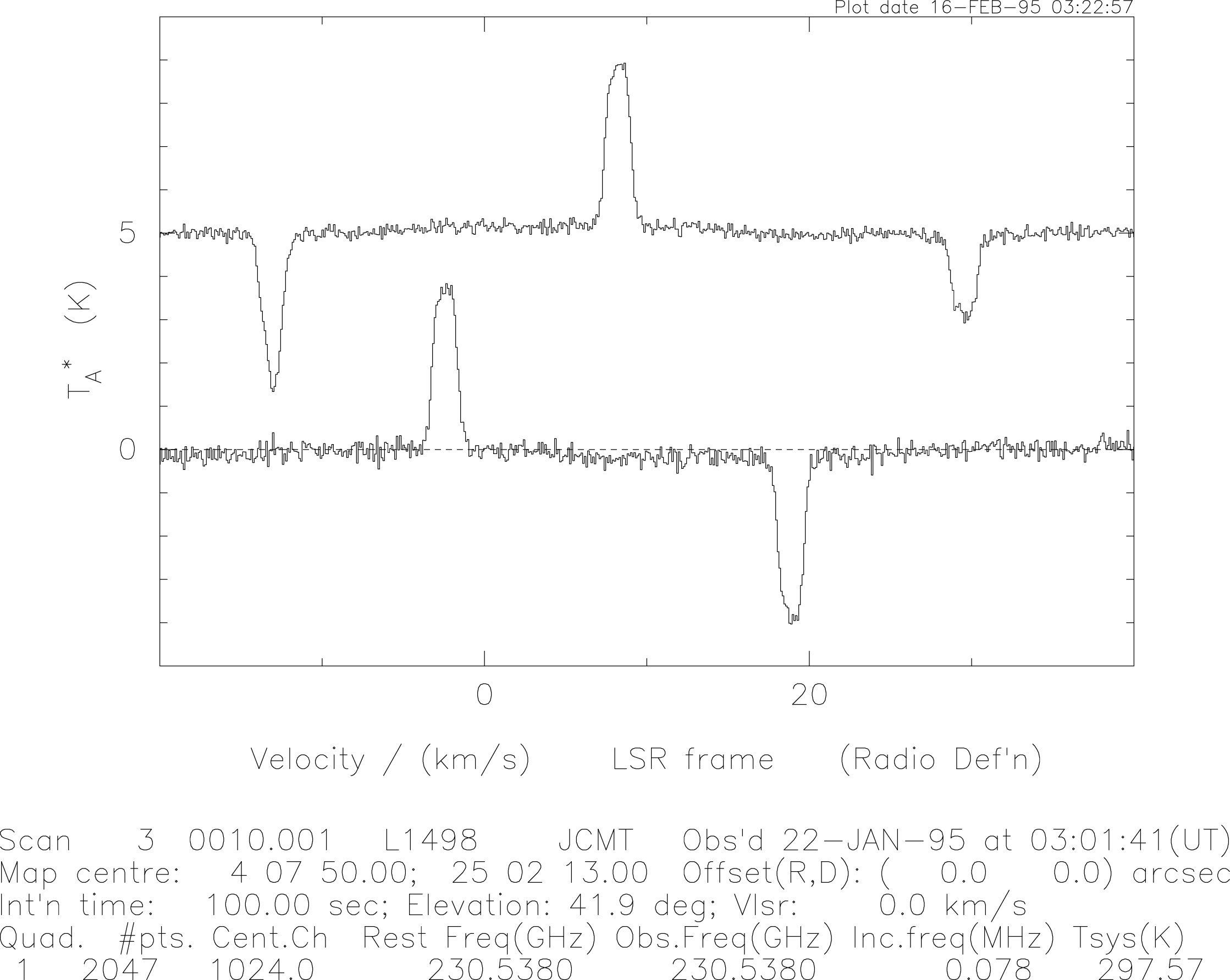
In practice one can expect a slowly-varying (and sometime large amplitude) sinewave across the band when observing in a frequency-switched mode. It may therefore be necessary to subtract higher-order polynomials from the baseline than with position- or beam-switching. In addition strong interference spikes can appear in the band, particularly when using A2. In other observing modes these will be largely cancelled out, but in the frequency-switched mode any such spike has the opportunity to appear twice. Such spikes may be accompanied by ‘ringing’ as a result of the Fourier transform applied to the data by the DAS. These problems should be taken into account during the data reduction.

Practical data reduction therefore consists of the following steps, some of which may be optional:

• Average all equivalent spectra together.
• If using more than one subband with the DAS merge the subbands together using the SPECX command das-merge. This step will not be needed if the spectra are taken with the AOSC.
• Apply Hanning smoothing to the spectrum if there is clear ‘ringing’ associated with spikes in the band.
• Remove interference spikes using e.g. rem-spike or set-chann in SPECX.
• There is a special procedure (fsw) to do the shifting and adding; it needs to be provided with the frequency shift you used during the observing; e.g. type:

  $>>$ fsw 8.1

  In this case the frequency switch was $\pm 8.1$ MHz.

  This takes the contents of the x-register (assumed here to be the result of the previous steps listed above) and replaces it with the shifted-and-averaged version. As noted within the procedure you may be asked to provide a frequency; this is the result of a software workaround for ‘slow-frequency switching’ (using receivers A2 and C2). To find out the frequency run SPECSUM and note the rest frequency given there for the data in question.

• Any residual baselines can now be removed with a polynomial (use f-p-b in SPECX) or composite (polynomial and sinusoidal; use f-c-b) function.
• Save the final result, once you are happy; you won’t want to do all this again.

3.18 Hardcopy and file output

If you really want to impress the tourists with your data you should plot out some spectra, or better still, maps, on the laserprinter, or make GIF files for WWW display. There are two ways to do this.

For spectra the easy way is to use the command laser. This command creates a plot file which may be sent to the local laser printer (defined in the setup of the node you are working at). The command see-plot has a similar effect to laser. In this case you provide the output device (terminal, printer, or null — the latter is a bit bucket); e.g.:

A more involved way involves first creating a plot file with which you can then do whatever you want. In this case first select the output medium you want using the command s-h-d:

As you can see there are quite a few possibilities, thanks to the use of up-to-date PGPLOT. In this case I wanted to change from a landscape GIF format to a color Postscript landscape plot. SPECX always gives the output file a default name; specx_pgplot.ps for Postscript, specx_pgplot.eps for Encapsulated Postscript, and specx_pgplot.gif for GIF files, for instance. Unix being what it is, this file will be overwritten every time you create a new plot file of the same type. Therefore if you want to save the plot file, rather than have it overwritten when you make the next plot, you should copy the generic file to a name of your choice; e.g.:

$>>$ $ cp specx_pgplot.ps myplotfile.ps

One cannot use the laser command for maps (see below).

3.19 Making Maps

Map making with SPECX is straightforward but it can be tedious if the map is quite large. It would be best if you tried using the following commands on a small map so that you get the idea and then use repetitive command files to create the large maps. Also, after you have made a map you can’t alter all the spectra in it without pulling them out, working on them and then replacing them. So if you want all the spectra smoothed or binned or whatever, make sure you do it before you make the map or you will have a job ahead of you. If this happens to you, it would probably be faster to just re-make the map.

3.19.1 Getting The Parameters Right

To make maps you have to create a map file first. Then you put spectra into the file. Map files are similar to data files except they always have read/write access. The command to start a map file is open-map-file.

Some words of advice first:

• You will need to provide the number of points in each spectrum (they should all be the same), which means you need to know this and have it set to a sensible number before you get going in a production mode. The number of points is given on a laser plot at the extreme lower left, and if you use the command print-spectrum-header (p-s-h will do) you can see the same information. Once you set the number of points in the map set-up, it will not be possible to stuff a spectrum containing fewer (if, say, you smoothed the data first) or more points into that map.
• The number of points selected is a crucial item as far as memory and disk space goes also. It is wise to limit the amount of the spectrum you want in your map to as few channels (200 or fewer may be enough sometimes) as is practical. Otherwise you may run out of disk space. With the large maps which can be made using the raster mode this is an important point. Limit the number of channels in the spectrum using the drop-channels command. See below.
• Only one map can be open at any one time. This means that it is very inefficient to transfer data from one map to another, using the commands get-spectrum-from-map and add-to-map in a command file. It is much better to hold the data in a SPECX data file and use that as an intermediary.

The key to all this is to experiment first with the data you plan to put in a map. Let’s illustrate this with an example of a real life situation.

The first thing to do is open a map file. The following dialog ensues once we type the command open-map-file:

Some explanation of the exchange is given below:

• On issuing the open-map command and a filename, one is prompted for a number of inputs if the map doesn’t already exist (if it does, that’s the end of the conversation, and the map is just opened with no further fuss).
• You give a map title and owner (note that these strings, like the ones associated with data files, should not contain spaces, etc).
• Next you specify whether the map centre is determined automatically from the first spectrum added to the map (this does not have to be the central point); if you answer negatively then you can provide a different central position. In the latter case note that the new map centre should be as closely as possible an integral number of pixels from the original observation centre in both coordinates.
• Next give the cell spacing and angle; these will probably be the same as those used during the observations. However, you could make the cell spacing half size, say, if you might want to fill in a sparse grid with more points later.
• Give the map size in numbers of the above map cells in both dimensions. Usually it is useful to choose a map size a little larger than the actual map. You might want to expand it later with more observations at the edges.
• Lastly, provide the number of channels in each spectrum. In this example I happen to know that I will want 247 points, having done some experiments beforehand. The baselines were a bit wiggly, so in this case I was more interested in fitting only part of the baseline, rather than saving disk space.

3.19.2 Map Files

To get data into the map, the command is add-to-map. This takes the spectrum in the X register and puts it in the map at the correct cell position. The first point you put in defines where the map centre will be (using the source coordinates and offsets), if you left that to be defaulted when you defined the map file setup with o-map; hence it doesn’t matter which map point you first put in the map. There is also a delete-from-map for removing data from the map. If you want to see a listing of what is in the map do list-map. If you want to take a spectrum out of a map to look at it or to do some other operation on it, use get-spectrum-from-map. And if you have gaps in your map, you can do interpolate-map and SPECX will try to fill in the holes.

So, here is the command file I used to add the spectra into the above map file:

In this case the map was made in the raster ‘on-the-fly’ mode. Because the integration time is limited to a few seconds in this case, the integration time per point was built up by making the same map 7 times, with calibrations before each scan, and a pointing part way through the series of maps. Hence I ended up with observations 17 thru 19 and 21 thru 24 inclusive. Each one consisted of 143 spectra (on a grid of 13 by 11 points). Hence the ‘do loop’ runs through each map point (143 times) (a) averaging the appropriate subscans together, (b) merging the subbands together, (c) chopping off the unused part of the spectrum, (d) fitting a quadratic baseline, and (e) adding the result to the map. To save time the screen display was not turned on. One can also do this kind of operation effectively with the read-gsd-raster and merge-files commands – see Section 3.19.4.

This file illustrates some more points about command file syntax.

• Comment lines can be inserted by starting the lines with !.
• The ‘n’ in the das-merge command inhibits subband offset adjustments; the ‘#’ is a ‘placeholder’ for the default channel drop.
• Two regions are chosen either side of the line emission for the polynomial fit. Note the method, using ^D (or ^Z), of terminating input to questions which have a larger number of possible answers than you need.

You may well find yourself wanting to replace all or part of your map subsequently. SPECX can be told to allow this, or not, using the set-map-access command. Thus:

Note that it is possible to set the positional tolerance of grid positions versus observed positions. The default is 0.7 pixel, but I prefer it tighter than that.

3.19.3 Dealing with lines in the other sideband

Quite often it happens that one feels quite clever in having set up a special frontend and DAS configuration in order to observe two or more lines in both sidebands simultaneously. That is the easy part; dealing with the data reduction, especially making a map of the line(s) in the other sideband requires a knowledge of the information in Section 3.16. As an example of the application of this, the following map-making file is offered as an example of how to make a map of CS 7–6 in the lower sideband, having observed CO 3–2 in the upper sideband. Various lines have been commented out, but can be brought into service as required:

3.19.4 The read-gsd-raster routine

Because map making can be slow due to system overheads, it is quite often useful to create a basic data file first from the various map observation GSD files. The routine read-gsd-raster provides this capability. You should have a file open first, to which the data can be written, and the routine reminds you to turn off the screen chatter with >> s-l-f n if you don’t want to see all the gory details.

Then, for example, the routine looks like this:

Then, away it goes. This routine does not fit baselines or truncate the noisy channels from the ends of the spectra, but it does das-merge the spectra as required. Subsequent application of the command merge-files allows data which should go in a single map cube to be combined. If one has two files containing grid, pattern, or raster data taken to a common centre merge-files will combine these data in a third file, averaging data taken at the same offsets. Thus this method is especially useful when one has data taken by several observers who have been confused about exactly where they should be observing, or when one has several observations of the same map grid. With the recent upgrade in speed resulting from improvements to the r-g-d routine this method does not confer any special advantage as to speed of application. It also tend to gobble up disk space due to the possibility of creating several large files rather than one.

3.19.5 Grid Spectra

One of the most useful ways of displaying small SPECX does maps is called grid-spectra. This produces postage-stamp size spectra on the screen lined up in the order they appear in the map. Figure 24 shows what happened when I gave the following commands:

Figure 24: Using the grid-spectrum command.

If the spectra does not come out right on the screen, try experimenting with set-map-size and set-map-scales. The map size determines the size of the window on the screen and the map scale determines what is in the window.

3.19.6 Contour Plots

Making contour plots with SPECX is easy. The command is contour-map. Figure 25 shows the result of the following commands on the map that is in Figure 24.

Figure 25: Contour plot of integrated emission over the line centre made using contour-map.

Again, if you have trouble getting what you want, adjust the map size and scale. Also, if you do set-contour-levels you can give it specific levels by saying no to the question about ‘Auto-contouring required’.

3.19.7 Color ‘grayscale’ images

Contour plotting is a bit boring; you can liven up the results by asking for grayscale plots using the command grayscale-map (gray is enough)⁹ Actually, most people make color ‘grayscale’ images these days; they are much more interesting. Thus:

This will produce a grayscale plot with overlaid contours. If you want to get rid of the contours, use set-gray, and answer ‘n’ in response to the query about contours:

The result is shown in Figure 26.

Figure 26: Grayscale plot of the same field

This really only works with a windowed terminal with a color monitor. However, the color table referred to allows a number of possibilities. Color table 4, for instance, produces a very nice blue thru yellow ‘grayscale’, and color table 5 is the “Cambridge colour spiral”. The best way to experiment with the option is to make a grayscale plot in interactive mode. Then, click on any point of the display window and type ‘h’ for ‘help’. A list of interactive options will appear in your SPECX window. SPECX really is very clever — I suggest you experiment with the options.

Once you have a plot you like on the screen, you should save it, or at least send it to the printer. To keep a recently made color Postscript file, say, you might do the following:

$>>$ $ mv specx_pgplot.ps myplot.ps
$>>$ $ lp -d color myplot.ps

This would send it to a printer named ’color‘.

3.19.8 Channel Maps

Another thing one can do is use channel-maps to make sequence of maps of the integrated or average emission in successive velocity slices. Figure 27 shows the result I got from the following:

The number of maps across the page can be chosen by you, but the auto option often does a very presentable job. In this case I wanted eight maps, four to a row.

Figure 27: Output of the channel-maps command

Most of these map facilities are touchy and few people get the picture they want the first time. Experiment with them though, it’s a good way to pass the time at the summit.

3.20 Data format conversion

As noted elsewhere the original spectral line data are written in GSD format. After processing by SPECX the output data, both spectrum datasets and maps, are in SDF format. For transmission to other sites it is possible to convert the data to either ASCII or FITS format via SPECX, if you don’t want them in your native format.

3.20.1 Conversion of older VMS SPECX data to Unix-readable format

Many people will have data reduced using the VMS versions of SPECX. These are in the wrong format to be read by Unix versions, and it is necessary to convert them to the correct format. The commands convert-vax-file and convert-vax-map are provided for this purpose.

• To convert a VMS SPECX data file type e.g.:
     >> c-v-f
     File name? ngc253.dat

  The new file will be named ngc253.sdf in this case.

  Note that one needs to give the full name of the file (ngc253.dat in this case), otherwise the following very serious-looking error will occur:

     >> c-v-f
     File name? ngc253
      --- openuf ---
          error in OPEN: FORTRAN i/o error #   1018
     Failed to open input file, IOSTAT =  1018
    !! HDS locator invalid: value=’ ’, length=15 (possible programming error).
    !  DAT_ANNUL: Error annulling an HDS locator.
     -- SPECX#010 -W- Error opening file --
     >>

  A similar error message will occur if the output filename already exists.

• Conversion of VMS maps (datacubes) proceeds along similar lines e.g.:
     >> c-v-m
     File name? mars_12

  In this example, the input map name was mars_12.map; the output map name will be mars_12_map.sdf. Note however an inconsistency with the c-v-f command: the full input map name is not required. Providing it will give an error e.g.:

     >> c-v-m
     File name? mars_12.map
      --- openuf ---
          error in OPEN: FORTRAN i/o error #   1018
     Failed to open input file, IOSTAT =  1018
     File name was mars_12.map.map
     -- SPECX#010 -W- Error opening file --
     >>  3

3.20.2 Conversion to ASCII files

If one wants to create a simple table of intensity versus the chosen abscissa (obtained using set-x), say, for subsequent manipulation using PGPLOT or MONGO this can be done using the command

$>>$write-ascii-spectrum

(w-a-s will do). The header information is minimal.

3.20.3 Conversion of single spectra to FITS format

To convert to a format readable by CLASS, it is first necessary to generate spectra arrays continuous in velocity/frequency space. Thus one must first have used the das-merge feature of SPECX for all but single-subband data of the DAS. There are two ways of doing this¹⁰.

• First write the spectra to a SPECX output file after applying das-merge and any other processing you want (such as baseline fits, binning etc). Then use the SPECX command

  $>>$tofits

  This will ask four questions: (a) which SPECX file number you want to use (hence the file must be open and read-permitted), (b) whether you want to use the original scan numbers or the sequence number in the SPECX file, and (c) the first and (d) the last scan in the input file to be processed by tofits. If you have single-position spectra (each with a distinctive integration number), or averages of the same, then choosing the original scan number option would probably be best. If your data are a sequence comprising a map, say, made with the grid, pattern or raster observing commands, then the scan numbers will be the same, but the subscan numbers will be incremented. In this case either the sequence number or the scan/subscan will do.

  The output filename has the following pattern in case one selects the option to imprint it with the original scan number:

    jcmt_nnnn_xxx.fits

  where nnnn is the scan number and xxx the subscan number. That is, the output file names might look like

         jcmt_0051_001.fits
         jcmt_0051_002.fits
                .
                .
                .
         jcmt_0051_015.fits

  in the instance of a 15-position map having been used for observation 51.

  If one chooses to imprint the filenames with the sequence number in the SPECX input data file, the subscan number is omitted: file names will look like jcmt_nnnn.fits.

  In both cases it will be useful to make a print-out of the input file using

  $>>$s-l-f f file.list
  $>>$in-f 1 l
  $>>$s-l-f t

  for example. In this case a complete (‘long’) listing of the SPECX input file number 1 is produced in file.list.

  To avoid digitization problems when converting FITS I4 integers tofits clips the data intensity values $I$ to be within the range $-500<I<+500$. The routine now also tells where it sits, so that one can copy and edit the procedure in case one wants to change the thresholds.

• GSD2FITS (or G2F): this routine (adapted from a SPECX script contributed by Christine Wilson) directly converts GSD files to FITS (with the above naming convention), where necessary using concat and das-merge (using default settings). It runs automatically without user intervention once started, and hence for all practical purposes appears as a disk-to-disk conversion. For example:
     >> g2f
    
     Routine to directly convert GSD DAS/AOSC files to FITS using CONCAT
     and DAS-MERGE if necessary.
    
     *** WARNING *** THIS ROUTINE IS DANGEROUS: data that need CONCAT
     and/or DAS-MERGE should really be inspected after these operations
     and before conversion to FITS, otherwise the DATA QUALITY may be
     severely compromised.
    
     /jcmt_sw/sun4_Solaris/specx/gsd2fits> First scan #? 51
     /jcmt_sw/sun4_Solaris/specx/gsd2fits> Last scan #? 59
    

  converts scans 51 through 59 (and all subscans) to FITS.

  The routine is designed to skip non spectral-line data. However, the user should be warned (as one can see!) against the blind use of this routine for data that needs concat and/or das-merge. I have had mixed results with it, and prefer to avoid it. The routine is usually fine for single-quadrant data, however.

3.20.4 Conversion of map cubes to FITS

SPECX has the capability to convert data cubes into FITS, either as velocity slices or complete cubes via the write-fits-map (w-f-m) and write-fits-cube (w-f-c) commands. The latter is a relatively recent addition and seems to work well generally.

w-f-m creates velocity slices i.e. maps of intensity versus position over a specified velocity range, say. Having decided on the velocity increment to use, and whether to use integrated or peak line strengths, one first opens a FITS file with the command open-fits. The name given the FITS file is quite literal; if you want the filetype to be .fits you have to specify it as shown in the examples below. Remember to close the FITS file with close-fits.

The following sequence is a typical example of how this would work:

w-f-c is also really very painless, and quite similar in mechanism to w-f-m:

Note the difference in size (given in bytes above) between map slices and cubes. The latter should be created carefully if you think diskspace is a problem. The above is a small (17 by 17 points, 700 channels) map, for reference.

3.21 Help

If you need help with some concept while using SPECX and you can’t find the answer here or in R. Padman’s manual, type help at the $>>$ prompt and go from there.

If you need a hint about a command, type the letter(s) you think the command should begin with. If you type set, for example, it will give you all the commands that begin with the word set in them.

There is a message which flashes by when you start SPECX. This message contains useful information on updates to the version you are using. If you want to see it again, type the command

$>>$ $ more $SYS_SPECX/specx_welcome.txt