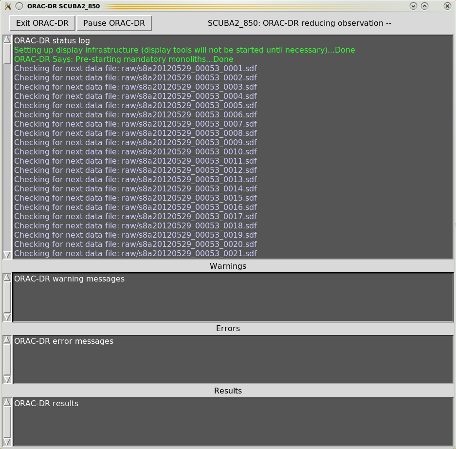
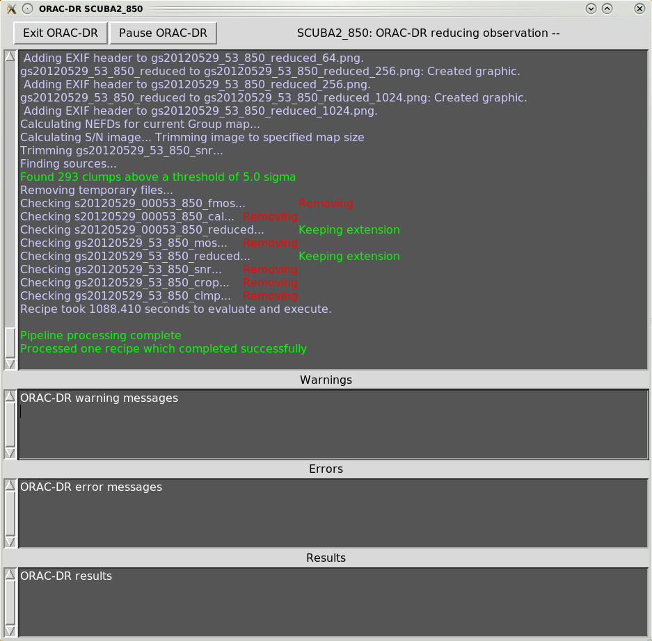
Figure 4.1: The Xwindows output from the Orac-dr pipeline showing the initial log—here we see the
pipeline is checking for the raw files.
REDUCE_SCAN
REDUCE_SCAN_CHECKRMS
REDUCE_SCAN_EXTENDED_SOURCES
REDUCE_SCAN_FAINT_POINT_SOURCES
REDUCE_SCAN_ISOLATED_SOURCE
FAINT_POINT_SOURCES_JACKKNIFE
SCUBA-2 data-reduction pipelines have been developed based on the existing Orac-dr pipeline (Cavanagh et al., 2008[3]) used for ACSIS. There are three distinct pipelines currently utilised by SCUBA-2. Users will likely only need to run the science pipeline. The other two pipelines are designed to run at the JCMT—the quick-look (QL) and summit pipelines. The latter two are run in real time at the JCMT during data acquisition.
The manual for the SCUBA-2 pipeline can be found at SUN/264, while the pipeline software comes as part of the Starlink suite. Data-reduction tutorials are available online1
The science pipeline will perform the following:
When a project is initially created and MSBs (Minimum Scheduling Blocks) are constructed using the JCMT Observing Tool, the PI can select a pipeline recipe to assign to the data. When the data are run through the science pipeline this recipe is then called by default. This can be overridden on the command line—see Section 4.4. Described below are the six main Orac-dr science recipes.
Note: the “dimmconfig*” files can be found in:
REDUCE_SCANConfiguration file: dimmconfig_jsa_generic.lis
This recipe uses the configuration file dimmconfig_jsa_generic for makemap, unless the sources is identified
as a calibrator in which case dimmconfig_bright_compact.lis is used and FCFs are derived from the map.
After all observations have been processed the data are co-added and calibrated in mJy/beam using the default
FCF. The noise and NEFD properties for the co-add are calculated and written to log files (log.noise and
log.nefd respectively). Finally, the Cupid task findclumps is run using the FellWalker algorithm (Berry,
2015[2]) to create a source catalogue.
REDUCE_SCAN_CHECKRMSConfiguration file: dimmconfig_jsa_generic.lis
This recipe is the same as REDUCE_SCAN, but includes extra performance estimations determined by
SCUBA2_CHECK_RMS (see Picard’s SCUBA2_CHECK_RMS). These extra metrics are written to a log file log.checkrms.
Running SCUBA2_CHECK_RMS in the pipeline, rather than as a standalone Picard recipe, allows it to calculate
results for co-added maps.
REDUCE_SCAN_EXTENDED_SOURCESConfiguration file: dimmconfig_bright_extended.lis
This is the recipe for processing extended sources. Multiple observations are co-added and the output map is calibrated in
units of mJy/arcsec.
This recipe also performs a source-finder routine; the results are written as a FITS catalogue (with file extension
.FIT) which can be read as a local catalogue into Gaia.
REDUCE_SCAN_FAINT_POINT_SOURCESConfiguration file: dimmconfig_blank_field.lis
This is the recipe for processing maps containing faint compact sources. This time the configuration file called
by makemap is dimmconfig_blank_field.lis and the map calibrated in mJy/beam. The output
map is further processed with a matched filter, then the S/N is taken to enhance point sources. A
map is written out at each step. This recipe also performs a source finder routine; the results are
written as a FITS catalogue (with file extension .FIT) which can be read as a local catalogue into
Gaia.
REDUCE_SCAN_ISOLATED_SOURCEConfiguration file: dimmconfig_bright_compact.lis
This is the recipe used for processing calibrator data. It can also be used for any map of a single bright, isolated source at the tracking position.
This reduction constrains the map to zero beyond a radius of 1 arc-min from the source centre. See Section 3.7.3
FAINT_POINT_SOURCES_JACKKNIFEConfiguration file: dimmconfig_blank_field.lis
This recipe uses a jack-knife method to remove residual low-spatial frequency noise and create an optimal
matched-filtered output map. The map-maker is run twice, first as a standard reduction using
dimmconfig_blank_field.lis (and calibrated in mJy/beam), and the second time with a fake source added to
the time series. This creates a signal map and an effective PSF map. A jack-knife map is generated from two
halves of the dataset and the maps are ‘whitened’ by the removal of the residual 1/f noise. The whitened signal
map is processed with the matched filter using the whitened PSF map as the PSF input. The data are calibrated
in mJy/beam using a corrected FCF. See Section 7.1.2 for a more-detailed description of this recipe and the files
produced.
Note: Data-reduction tutorials are available online.
| Step 1: | Initialise ORAC-DR
For 850-m data, this is done by: For 450-m data, this is done by: |
|---|---|
| Step 2: | Set environment variables
These ensure the data are read from and written to the right places. Many are set automatically when the pipeline is initialised but others must be set manually. Details of the optional variables are given in SUN/264 but the three main ones are:
Example: Setting
and for Bourne shells (sh, bash, zsh): |
| Step 3: | Run the pipeline
This is done by: where the list of files that you wish to reduce can be an individual or multiple observations (one per line in a text file, with full path names). |
When executing the Orac-dr command, unless “-nodisplay” is specified, various graphical windows may appear showing the pipeline results. Also with the default “-log” option (including “x”) a new Xwindow will appear which will contain the pipeline output, as shown in Figures 4.1– 4.4.
Orac-dr’s behaviour can be changed on the command line. For help simply type
To run the pipeline and obtain all messages from the Starlink engines (rather than just Orac-dr messages) you will need to run with verbose (recommended)
To run the pipeline and have the results sent to the screen (s) and to a file (f—the file produced is usually called
.oracdr_NNNN.log where NNNN is the current process ID. It is written to $ORAC_DATA_OUT and is a hidden
file) is specified using the -log command.
You can override the recipe set in the header by listing any different one on the command line when starting Orac-dr. For example
You can find out which recipe is set in the data header via the FITS header RECIPE keyword in any of your raw
files. For example both of these options will return the same result (ensure KAPPA commands are available
before running):
Although each recipe calls one of the standard configuration files you can specify your own. You will need to
create a recipe parameter file. This file will set the parameter MAKEMAP_CONFIG to be your new configuration file.
The first line must be the name of the recipe used in the reduction.
For example, to run the pipeline with REDUCE_SCAN_CHECKRMS with a configuration file called myconfig.lis, the
recipe parameter file (mypars.ini) will look like this.
Then run the pipeline calling the parameter file via the -recpars option.
To supply both a new configuration file and a different set of clump-finding parameters we would update the
parameter file mypars.ini to look like:
Other options we can change in the parameter file include—changing the pixel size
changing output units to mJy/beam
changing output units to mJy/arcsec
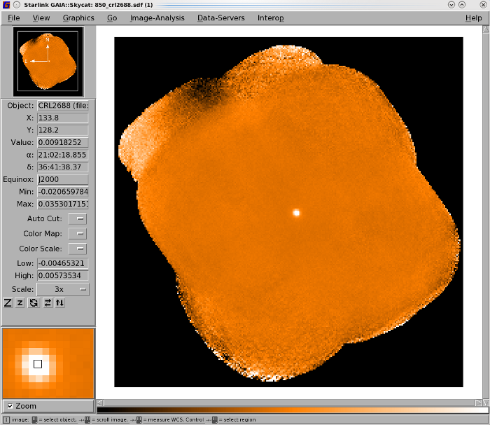
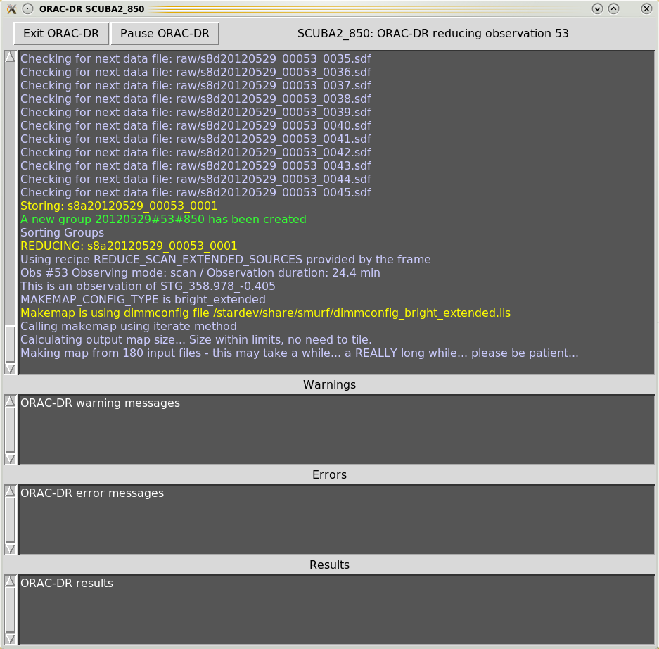
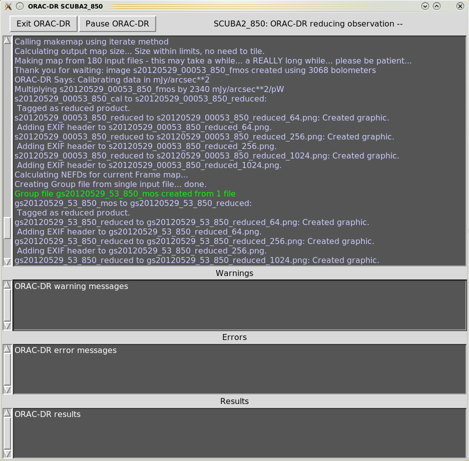
Once the map-maker has completed you can open your output map using Gaia (see Figure 4.5). The excerpt in Chapter 5 shows the output written to the terminal as you run the map-maker. There are a number of clues in this output that indicate the status of the reduction.
Continuous chunk 1 / 1.
Chunking is where the map-maker processes sub-sections of the time-series data independently
and should be avoided if possible—see the text box on Chunking.At the beginning of the reduction, the main purpose of QUALITY flagging is to indicate how many bolometers
are being used. In the example above you can see that from a total of 5120 bolometers, 1842 were turned off
during data acquisition (BADDA). In addition, 136 bolometers exceeded the acceptable noise threshold (NOISE),
while tiny fractions of the data were flagged because the telescope was moving too slowly (STAT) or the sample
are adjacent to a step that was removed (DCJUMP).
The total number of bad bolometers (BADBOL) is 1984. Accounting for these, and the small
numbers of additionally flagged samples, 3128.22 effective bolometers are available after initial
cleaning2.
After each subsequent iteration a new ‘Quality’ report is produced, indicating how the flags have changed. An
important flag that appears in the ‘Quality’ report following the first iteration is COM: the DIMM rejects
bolometers (or portions of their time series) if they differ significantly from the common-mode (average) of the
remaining bolometers.
You may note that compared with the initial report, the total number of samples with good ‘Quality’ (Total
samples available for map) has dropped from 18634826 to 18273302 (about a 2 per cent decrease) as
additional samples were flagged in each iteration.
Be aware that some large reductions may take many iterations to reach convergence and you may find significantly fewer bolometers remaining resulting in higher noise than expected.
The convergence criteria maptol is updated for each iteration. The convergence can be checked from the line
reporting
smf_iteratemap: *** NORMALIZED MAP CHANGE: 0.10559 (mean) 2.81081 (max)
The number to look out for is the mean value of the NORMALIZED MAP CHANGE. This will have to drop
below your required maptol for convergence to be achieved.
The default configuration file used in this example executes a maximum of
five iterations, but stops sooner if the change in maptol drops below 0.05 (i.e.
numiter =5).
In this example it stops after five iterations.
Ctrl-C. The map-maker will complete the
iteration then write out a final science map. Entering Ctrl-C twice will kill the process immediately.
The pipeline will produce a group file for each object being processed. If the pipeline is given data from multiple nights, all those data will be included in the group co-add using inverse variance weighting.
The final maps in your output directory will have the suffix _reduced. Maps will be made for individual
observations, which will start with an s for “SCUBA-2” (e.g. s20140620_00030_850_reduced.sdf). Group
maps, which may contain co-added observations from a single night, are also produced which have the prefix
gs for “group SCUBA-2” and the date/scan of the first input file (e.g. gs20140620_30_850_reduced.sdf).
Note: A group file is always created, even if only a single observation is being processed.
Additionally, PNG images are made of the reduced files at a variety of resolutions.
Another useful feature is that the pipeline will generate log files to record various useful quantities. The standard log files from reducing science data are:
log.noise—noise in the map for each observation and the co-add (calculated from the median of
the error array), and
log.nefd—NEFD calculated for each observation and for the co-added map(s).
log.removedobs—list of observations removed from each group (e.g. due to failing QA).The JCMT Science Archive is hosted by The Canadian Astronomy Data Centre (CADC). Both raw data and data processed by the science pipeline are made available to PIs and co-Is through the CADC interface (https://www.cadc-ccda.hia-iha.nrc-cnrc.gc.ca/en/jcmt/).
To access proprietary data you will need to have your CADC username registered by the EAO and thereby associated with the project code. Please contact your friend of project or helpdesk@eaobservatory.org to register your account.
An important search option to be aware of is ‘Group Type’, where your options are Simple, Night, Project and Public. Simple (which becomes ‘obs’ on the result page) is an individual observation; night means the group file from the pipeline (these may or may not include more than one observation; the ‘Group Members’ value will tell you); and the project option is generated if an entire project has been run through the pipeline and identical sources across the project are co-added into master group files.
1https://www.eaobservatory.org/jcmt/science/reductionanalysis-tutorials/
2The fractional number is due to time-slices being removed during cleaning. The number of bolometers is then reconstructed from the number of remaining time-slices.