3 Theory support

Starlink provides access to computer algebra by supporting the Maple package. You might have access to Maple on your own Starlink node, but if not, you may use it on the machine star.rl.ac.uk, if you have an account there. If you are a Starlink user, you should apply for an account by mailing star@star.rl.ac.uk.

Maple allows you to enter mathematical expressions using a fairly natural syntax, substitute into them, simplify them, differentiate and (with limits) integrate them, and finally go on to graph them. As an added bonus, you can also produce output in C, Fortran and LaTeX.

We start up Maple, and enter an expression for a gaussian. Maple makes an attempt to display the result intelligibly. If we had ended the expression with a colon rather than a semicolon, Maple would have suppressed the display. Note that undefined variables represent themselves, and that Maple knows that exp is the exponential function, so that it knows, for example, how to differentiate it.

Then differentiate the gaussian, and assign the result to gid. The result is something you’re happy not to have had to work out yourself.

If that the purpose of this was to do a calculation somewhere, you might want to code this expression in Fortran. Doing this by hand would be error-prone, but Maple can produce output in Fortran as well as this ‘prettyprinted’ style.

The optimized argument tells Maple to try to produce Fortran code without repeated subexpressions. You can save this to a file with the expression fortran (gid, filename=‘gaussian.f‘, optimized); You can produce output in C as well, though because the identifierC is potentially such a common one, you must explicity load the C library first.

There are two things to note here. The first is that we have renamed the expression gid on the fly. The second is that the expression for t4 is not the most efficient — it is very bad to use the pow() function for raising expressions to small integer powers: much better would be t4a=xc-x0; t4=t4a*t4a;, as has happened automatically for t10.

Maple has done the correct thing with the cosine and sine functions, and with the

θ

variable, and it has got all the braces matching correctly, but it has expressed the exponential as a simple e-to-the-power which will look rather ugly (as well, the exponential should be written with \mathrm{e}).

SUN/107 provides an introduction to Maple, and SGP/47 is a comparison of Maple and Mathematica. Also, the Maple manual and tutorial are very clear. There is help within Maple (type ?intro), and this gives enough information to get you going. Maple’s web pages are at http://www.maplesoft.com/, but they don’t currently (December 1998) give a lot of tutorial help. See also the example Maple program in A.7.

As a final point, don’t fall into the common trap of thinking that because you’ve produced your result using computer algebra, it must be right. This is as false of computer algebra as it is of numerical programming — be inventive in thinking of cross-checks.

3.2 Data visualisation

Starlink supports two data visualisation packages, IDL and DX, but for relatively simple graphing of simple results, gnuplot will probably produce acceptable results in rather less time.

The package SM, which is a descendent of Mongo, has numerous adherents, but I don’t propose to discuss it, partly because I’ve never used it, partly because it’s not part of Starlink’s base set and so is not available at all sites, but mostly because if gnuplot runs out of steam, you might as well go straight to IDL, which is easily available through Starlink.

SG/8, “An Introduction to Visualisation Software for Astronomy”, is an overview of visualisation systems, which mentions both IDL and DX.

3.2.1 gnuplot

Gnuplot is valuable because it’s so simple — easy things can be done easily. If you want to graph an equation or plot some data, and produce postscript output, then you’ll probably do it faster, from a standing start, than someone using one of the beefier packages. Its weaknesses are that it can’t easily do very complicated or fancy visualisations (that is, it doesn’t try to take over the world), and it deals naturally only with ASCII data in columns. It is scriptable, but I wouldn’t fancy programming anything complicated with it.

Start it up with the simple command gnuplot. Once it’s started, you can give it commands as simple as

to produce a plot of the sine function with default ranges, or you can give it a range and specify a line type as follows

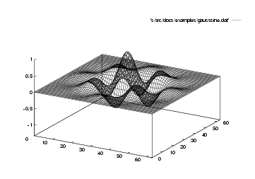
Gnuplot can also graph data files. The example file gausssine.dat consists of two columns of

64 \times 64

values. It can be plotted in gnuplot with the commands:

This produces the EPS file shown in 3.1. The file has a blank line after each block of 64 numbers. Gnuplot interprets this as a signal that this is the end of a ‘row’ of a matrix (a standard gnuplot gotcha is that is must be a completely blank line, with no whitespace). You can plot the surface represented by the second column, with the clause using 2 to splot. Gnuplot can read more generally formatted data, but that’s already stepping towards advanced usage.

Figure 3.1: File gausssine.dat, displayed with gnuplot

There is good help within gnuplot, available by typing help.

3.2.2 IDL

IDL is much more powerful and flexible than gnuplot, and has a correspondingly longer learning curve. It’s never been accused of being elegant, but with only a bit of headbanging, I’ve always managed to get it to do what I wanted (I’ve always seen it as reminiscent of Fortran in this respect).

Several missions have used IDL as the language in which they have written their data-analysis software, and Starlink is currently experimenting with providing IDL interfaces to important Starlink applications, which is possible because IDL can link to codes written in languages such as Fortran or C. IDL is moving towards being a core facility at Starlink sites.

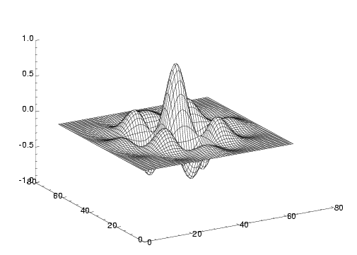
IDL displays data in arrays as part of a generic set of array manipulations. For example, the data in the file gausssine.dat was produced by the following sequence of IDL commands:

  x=(findgen(64)-32)^2
  d=fltarr(64,64)
  for i=0,63 do d(i,*)=sqrt(x+(i-32)^2)
  a3=exp(-(d/15)^2)
  s=sin(findgen(64)/63*5*3.141592657)
  s2=s#s
  m=s2*a3

The function findgen(N) returns a float array (indexed from 0 to $N - 1$ ) in which the value of each element is the same as its index; performing an arithmetic operation such as subtraction or exponentiation on an array performs it on each element of the array; fltarr declares an array of floats of the specified dimensions; the array reference d(i,*) refers to the entire i’th row of d; the operator # forms the direct product of the two vectors. The result of this is to set d to be an array where each element is the euclidean distance from element (32,32)¹.

Once we have the data in the array m, we can produce a surface plot with surface,m, and then go on to annotate it, rotate it, shade it, contour it, with the large collection of options and parameters to the surface command. We can produce PostScript output with the following sequence of commands:

    !p.font=0             ; use postscript fonts rather than IDL outlines
    set_plot, ’ps’        ; use the postscript output driver
    device, /encap, filename=’gausssine-idl.eps’
                          ; produce encapsulated postscript
    surface, m
    device, /close        ; close the file

This produces the EPS file shown in 3.2. A minor, but persistent, irritation with IDL is that, although its input and output facilities are as flexible as, say, Fortran’s (which they closely resemble), it doesn’t come with a function for dealing with the common case of data printed out in columns (the only case gnuplot naturally deals with). Fortunately, such a function is not only easy to write, but a useful example, too. See A.8.

Figure 3.2: File gausssine.dat, displayed with IDL

IDL comes with rather good manuals, the reference parts of which are available on-line by typing ? at the IDL prompt.

See appendix B of SUN/55 for a description of how to import data in the Starlink NDF format into IDL.

3.2.3 DX

IBM’s Data Explorer is also available on some Starlink machines. I don’t have personal experience of it, but there is a Starlink manual for it in SUN/203, “SX and DX — IBM data explorer for data visualisation” and a Starlink DX cookbook in SC/2.

In his overview of visualisation systems in SG/8, Clive Davenhall says of DX:

IBM Data Explorer (DX) is a general-purpose software package for data visualisation and analysis. It employs a data-flow driven client-server execution model and provides a comprehensive range of data manipulation, visualisation and display functions. Visualisations can be generated using a visual programming editor or a text-based scripting language. DX is the visualisation package recommended by Starlink, particularly for three-dimensional scalar and vector data. Starlink has produced a set of enhancements to DX. If you are using DX at a Starlink site then these enhancements should be available automatically. The use of DX at Starlink sites and the Starlink enhancements to DX are documented in SUN/203.

3.2.4 PGPLOT

The above recommendations describe standalone packages which work on data produced by your code in a separate step. An alternative route is to incorporate the plotting facilities within your program, and the recommended way of doing this is by using the PGPLOT library.

The library, which was written to support astronomical applications, consists of a collection of high-level routines for producing plots, maps and images either on-screen or as Postscript to a file. Refer to SUN/15, “PGPLOT — Graphics Subroutine Library” for further details, or to the PGPLOT home page at .

Note that there are two versions of PGPLOT currently available on Starlink, ‘native’ PGPLOT, and a Starlink version which uses GKS. The latter is being deprecated, with a view to being ultimately phased out, and this will affect how you link your program against the library. At the time of writing (December 1998), the way in which the dual versions will be supported has not been finalised; ask your system manager for advice.

3.3 Producing images

If you wish to include images in your LaTeX output, do so using the standard graphics package. That is, include in your file the command \usepackage{graphics} (if you’re obliged to use the old LaTeX2.09, you can use the epsf option to the document style). Include the graphics with the command \starincludegraphics{file.eps}. So how do you produce the postscript?

An important point is that the postscript should be encapsulated postscript. This is postscript intended to be incorporated within another document: it has a BoundingBox comment at the top of the file, and typically has the extension .eps.

See 3.2 for details of how to produce EPS plots from gnuplot and IDL.

If it’s diagrams you want to produce, then xfig has its adherents. There’s a large manual page for xfig, but you can do pretty well just starting it up, and pointing and clicking.

If point and click isn’t your style, try MetaPost. This is a variant of Knuth’s MetaFont (which is used for designing TeX fonts), which produces postscript instead. To produce a document using MetaPost, you produce a text file specifying the objects you want to draw and their spatial relationships. It can be hard work, but the results can look very good. If you wished to automate producing diagrams, perhaps because you want to produce a set of diagrams which are systematically different, then MetaPost could very well help you with this. See .../texmf/doc/metapost under the (Starlink) TeX tree for further details.

¹IDL experts will know that the common IDL idiom for this is d=shift(dist(64),32,32), but have you ever actually compared dist with its documentation? The documentation for dist suggests that this idiom wouldn’t work, but the function’s actual behaviour seems to (substantially) depart from the claimed behaviour in exactly the right way.

←Prev
Theory and Modelling Resources Cookbook
Next→
TOC ↑

Chapter 3
Theory support

3.1 Computer algebra

3.2 Data visualisation

3.2.1 gnuplot

3.2.2 IDL

3.2.3 DX

3.2.4 PGPLOT

3.3 Producing images

Chapter 3Theory support

3.1 Computer algebra

3.2 Data visualisation

3.2.1 gnuplot

3.2.2 IDL

3.2.3 DX

3.2.4 PGPLOT

3.3 Producing images

Chapter 3
Theory support