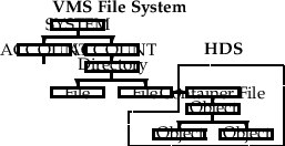
Figure 10.1: The relationship between VMS and HDS.
HDS — the Hierarchical Data System — is one of the most powerful features of ADAM. It is implemented as a set of subroutines which are of much more interest to the programmer than the user of the programs. Nevertheless, as a user it is necessary for you to know something of the system in order to make the best use of your data. HDS is about storing astronomical data in a compact, flexible and efficient way. It recognises that observations are often complex — possibly consisting of a data array (in 1, 2, 3, or even more dimensions), together with variable amounts of ancillary data — calibrations, errors, telescope and instrument information, observing conditions, and so on. The way HDS handles this complexity bears some similarities to the way VMS handles directories and files.
HDS files are known as container files and by default have the extension ‘.SDF’. They contain data objects which will be referred to simply as objects when the context makes clear what sort of object it is. An object is an entity which contains data or other objects. This is the basis of the hierarchical nature of HDS and is analogous to the VMS concepts of file and directory — a directory can contain files and directories which can themselves contain files and directories and so on (Figure 10.1). An object possesses the following attributes:
HDS allows great freedom in specifying names and types, but standards have been laid down (see Section 10.2) to encourage portability of data and applications. Name: An object is identified by its name. This must be unique within its own container object. This is in contrast to VMS where different files in the same directory may be distinguished by their version numbers. A name is written as a character string containing any printing characters. Spaces, tabs and so on are ignored and alphabetic characters are capitalised. There are no special rules governing the first character (i.e. it can be numeric). When referring to components of objects, the following syntax is used:
where C is a component of B, and B is a component of A, which is the top-level object in the container file. Some specific examples of names are given at the end of this section. Type: The type of an object falls into one of two classes:
Structure objects contain other objects called components. Primitive objects contain only numeric, character, or logical values. Objects in the different classes will be referred to simply as structures and primitives, while the more general term object will refer to either a structure or a primitive. Structures are analogous to VMS directories — they can contain a part of the hierarchy below them. Primitives are analogous to VMS files — they are at the bottom of any branch of the structure.
The primitive types defined in HDS are shown in Table 10.1.
| HDS Type | VAX Fortran Type | Length in Bits |
| _INTEGER | INTEGER | 32 |
| _REAL | REAL | 32 |
| _DOUBLE | DOUBLE PRECISION | 64 |
| _LOGICAL | LOGICAL | 32 |
| _CHAR[*N] | CHARACTER*N | 8*N |
| _UBYTE | BYTE | 8 |
| _BYTE | BYTE | 8 |
| _UWORD | INTEGER*2 | 16 |
| _WORD | INTEGER*2 | 16 |
The first five of these types are referred to as standard data types. The _UBYTE type provides a value range of 0 to 255; the _UWORD type provides a value range of 0 to 65535. The others are as for Fortran 77. Examples of structure types are IMAGE, SPECTRUM, INSTR_RESP etc. Their names don’t begin with an underscore, so the system and the programmer can easily distinguish between primitives and structures. A type is written as a character string with the same rules as for name, except that an asterisk can only appear if the first character is an underscore (i.e. it is a primitive), and also a type can be blank. Shape: Every object has a shape or dimensionality. This is described by an integer (the number of dimensions) and an integer array (the size of each dimension). A scalar, for example a single number, has by convention a dimensionality of zero, i.e. number of dimensions is 0. A vector has a dimensionality of 1, i.e. number of dimensions is 1 and the first element of the dimension array contains the size of the vector. An array refers to an object with 2 or more dimensions; currently a maximum of 7 dimensions are allowed. Objects may be referred to as scalar primitives or vector structures and so on. State: The state of an object specifies whether or not its value is defined. In routines it is represented as a LOGICAL variable where .TRUE. means defined and .FALSE. means undefined. Group: In order to access an object, it is first necessary to obtain a locator, a sort of pointer which can then be used to address the object. When the program no longer needs to access the object, the locator should be annulled. A locator is analogous to a Fortran logical unit number (but is actually a character variable, not an integer). Any number of locators can be active simultaneously. The group attribute is used to form an association between locators so that they can be annulled together. A group is written as a character string whose rules of formation are the same as for name. Value: When an object is first created it contains no value, somewhat like an empty file. It must be given a value in a separate operation. A value can be a scalar, vector, or an array. The scalar or the elements of the vector or array must all be of the same type and can be primitives or structures. The rules for handling character values are the same as for Fortran 77, i.e. character values are padded with blanks or truncated from the right depending on the relative length of the program value and the object. Illustration: To fix ideas, look at the example of an NDF data structure in Figure 8.2. The following notation is used to describe each object:
where ‘(dimensions)’ only appears when describing vectors or arrays. Each level down the hierarchy is indented.
Suppose an object with this structure were stored in a (container) file called EXAMPLE.SDF, then we can refer to components of this object by names such as:
A major preoccupation of Starlink since its inception has been to design a data storage format which is both standard and yet which can accommodate most of the things which one might wish to store. (This is a weak point with most software environments in astronomical use at present.) One of the practical problems with unfettered HDS is that it is too flexible. The solution adopted, NDF (Extensible N-dimensional-Data Format), provides a more limited set of designs, but still implemented using HDS. It is described in awesome detail in SGP/38.
In essence, NDF defines a set of standard data objects. Not all of them must be present in an NDF object, but no others will be processed. Non-standard items are handled in a standard way by using self-contained extensions. There are defined locations for items such as the main data array, axes, title, units etc. The only mandatory item is the main data array; all other items are optional!
All this means that the user can be certain that no properly written application will mess up his data, and there is a very good chance that all the useful information will be properly used. (For the programmer, the huge advantage of this system is that he doesn’t need to know the details of the format at all! A comprehensive set of routines is available to access the standard components of an NDF. These are described in Section 21.2.1 and (more fully) in SUN/33.)
ADAM_EXAMPLES:EXAMPLE.SDF is file containing an NDF object which contains all the standard NDF components and also has a Figaro extension. Such a file is often referred to as an ‘NDF file’, or even as just an ‘NDF’. The structure of the file, as revealed by:
is shown in Figure 8.2.
The components of an NDF are described below. The names (in bold type) are significant as they are used by the NDF access routines to identify the components.
1The file was converted to an NDF using the CONVERT command DST2NDF.