Processing math: 100%

Part III
Worked Examples

 10 Introduction
 11 Reducing Hydra Data Using IRAF
 12 Reducing FLAIR Data Using IRAF
  12.1 Setup file customisation
 13 Reducing 2dF Data Using 2dFDR
 Acknowledgements
 References

10 Introduction

This part of the cookbook provides a set of worked examples of reducing fibre spectroscopy observations from various instruments. The examples are:

The example of reducing Hydra data is available as part of the documentation for IRAF. The procedure is similar to, but simpler than, the procedure for reducing FLAIR data. Consequently it is sensible to work through the Hydra example before trying the FLAIR one.

All the examples assume that the requisite software is already installed at your site and ready for use. If the software is not available at your site then Section 7 describes how to obtain it. Note, however, that you will often require the assistance of your site manager to install the software.

Copies of the data files used in the examples are provided so that you can work through them yourself. On Starlink systems they are kept in directory:

  /star/examples/sc14

Alternatively they can be retrieved by anonymous ftp from Edinburgh. The details are as follows:

site: ftp.roe.ac.uk
directory /pub/acd/misc
file sc14.tar.Z

Reply anonymous to the ‘Name’ prompt and give your e-mail address for the password. Set ftp to binary mode before retrieving the file. The file is a compressed tar archive and should be decompressed with the Unix command uncompress (sic).

In order to work through the examples you should use a display capable of receiving X-output (typically an X-terminal or a workstation console). Strictly speaking the software will run on a black-and-white device, but realistically you need a colour display. Before starting you should ensure that your display is configured to receive X-output.

Finally, the examples show only some of the features of the various packages used. In all cases they have additional features which are not described here. You should see the appropriate user manuals for full details.

11 Reducing Hydra Data Using IRAF

Hydra is a fibre spectrograph available at the Kitt Peak National Observatory (KPNO), Tucson (see, for example, Barden et al.[7]). Observations acquired with it are usually reduced using the IRAF task dohydra. dohydra is very similar to the IRAF task dofibers which is used to reduce FLAIR and WYFFOS/AUTOFIB2 data. A worked example of using dohydra is available as part of the IRAF documentation. This example is similar to, though simpler and easier than, the example of reducing FLAIR data given in Section 12, below. Thus, it is sensible to work through the Hydra example before trying the FLAIR one, even though you are unlikely to observe with Hydra.

Before trying the Hydra (or FLAIR) example you should already be familiar with the rudiments of IRAF and have an ‘IRAF directory’ prepared which you will use for running IRAF. If you are not au fait with IRAF then you must familiarise yourself with it before proceeding; SG/12: An Introduction to IRAF[34] is a convenient starting point.

The dohydra tutorial is available at URL:

http://www.starlink.ac.uk/iraf/web/tutorials/dohydra/dohydra.html

You can simply follow the instructions given and there is no need to repeat them here. There are, however, a couple of caveats which you should be aware of.

(1)
The sequence of IRAF packages to load given in the tutorial is slightly incorrect. The correct sequence is:
  noao
  imred
  hydra
(2)
An IRAF script is provided with the present cookbook to automatically set all the dohydra parameters recommended in the tutorial. It is available as file:
  /star/examples/sc14/hydra/hydrasetup.cl}

You should make a copy of this file in your IRAF home directory. Then from the IRAF command line type:

  task  $hydrasetup=home$hydrasetup.cl
  hydrasetup

For information the script echoes the values that it sets to the IRAF command line.

12 Reducing FLAIR Data Using IRAF

FLAIR observations are usually reduced using IRAF (see Section 7.3.1) and this example is a simple demonstration of the procedure. The reduction of FLAIR data is documented in the manual FLAIR Data Reduction with IRAF[20]. The present example gives all the steps involved in a simple reduction but nonetheless you will find it useful to have a copy of the manual to hand as you work through it for further explanation of each step and future reference.

The example assumes that you are familiar with the rudiments of IRAF and already have an ‘IRAF directory’ prepared which you will use for running IRAF. If you are not au fait with IRAF then you must familiarise yourself with it before proceeding; SG/12: An Introduction to IRAF[34] is a convenient starting point. Reducing FLAIR observations with IRAF is similar to, but more complicated than, reducing Hydra observations, which was described in the previous example (Section 11, above). Consequently, it is sensible to work through the Hydra example before trying the present one.

The data used in this example are observations of some early-type stars in the direction of the Galactic centre. The stars are in the magnitude range 12 to 16 and the spectra cover the wavelength range 4000–4600Å. These data are unusual in that most FLAIR observations are of external galaxies. Nonetheless they can be used to illustrate the reduction procedure, which is as follows.

(1)
Make your IRAF directory your current directory. All the files used in the example are available in directory /star/examples/sc14/flair. Copy these files to your IRAF directory:
  cp  /star/examples/sc14/flair/* .

The various files will be introduced as they are required. However, they are all listed in file 0FLAIR.LIS.

(2)
Start IRAF. See SG/12 for further details. You should use the customisation file
loginuser.cl
provided with SG/12 to ensure that IRAF is configured correctly to handle the large headers in FLAIR files (if you do not use this customisation file you may or may not encounter problems, depending on how IRAF is configured at your site).
(3)
Load all the various IRAF packages and sub-packages which are required. Type:
  noao
  imred
  ccdred
  specred
  astutil
  flair

If any of the packages are not found then the most likely explanation is that they are not installed at your site; ask your site manager to install them. See Section 7.3 for details of how to obtain the FLAIR software and SG/12 for the standard IRAF packages.

(4)
Several IRAF tasks have to be run in order to reduce FLAIR data and for most of them ‘hidden’ parameters have to be set. The FLAIR manual[20] gives the necessary details. However, for convenience, the script flairsetup.cl is provided with the example. It simply sets all the required values. It is correct for the example data and can simply be used unaltered. However, if you wish to use it with your own data there are couple of items which may need to be changed. Section 12.1 gives the details. To define and run the script simply type:
  task  $flairsetup=home$flairsetup.cl
  flairsetup

For information the script echoes the values that it sets to the IRAF command line.

(5)
FLAIR data are provided as FITS files, of file-type .fts. They must be converted to the IRAF OIF format. Rather than specifying all the file names individually they have previously been listed in file fits.lis provided with the example (you might like to examine this file and check that it is just a list of file names). The procedure for making the conversion differs slightly depending on which version of IRAF you are using:
IRAF version 2.10
:  
  rfits ~ @fits.lis  1  rawflair
IRAF version 2.11
:  
  rfits  @fits.lis  0  rawflair
(6)
Some twenty-four files are included in the example, comprising a mixture of bias, flat field, arc and object observations. You need to know which file corresponds to which type of observation. This information may be available from your observing log. However, if necessary it can be extracted from the data files themselves. Type:
  imhead  rawflair*.imh  >  heads.txt

Here task imhead extracts the header information and the IRAF cl Unix-like output redirection mechanism is used to write it to file heads.txt. The contents of this file should be:

  rawflair0001.imh[420,578][short]: Bias
  rawflair0002.imh[420,578][short]: Hg-Cd
  rawflair0003.imh[420,578][short]: F454-1
  rawflair0004.imh[420,578][short]: F454-2
  rawflair0005.imh[420,578][short]: F454-3
  rawflair0006.imh[420,578][short]: F454-4
  rawflair0007.imh[420,578][short]: F454-5
  rawflair0008.imh[420,578][short]: Rb
  rawflair0009.imh[420,578][short]: Rb
  rawflair0010.imh[420,578][short]: Hg-Cd
  rawflair0011.imh[420,578][short]: Hg-Cd
  rawflair0012.imh[420,578][short]: Dome flat
  rawflair0013.imh[420,578][short]: Dome flat
  rawflair0014.imh[420,578][short]: Dome flat
  rawflair0015.imh[420,578][short]: Bias
  rawflair0016.imh[420,578][short]: Bias
  rawflair0017.imh[420,578][short]: Bias
  rawflair0018.imh[420,578][short]: Bias
  rawflair0019.imh[420,578][short]: Bias
  rawflair0020.imh[420,578][short]: Bias
  rawflair0021.imh[420,578][short]: Bias
  rawflair0022.imh[420,578][short]: Bias
  rawflair0023.imh[420,578][short]: Bias
  rawflair0024.imh[420,578][short]: Bias

A copy of the output is also provided in file flairheads.txt for comparison. It is obvious from this output which file contains which sort of observation.

(7)
The header information in the raw FLAIR data contain some oddities which must be fixed-up before the data can be processed with IRAF. The utility fixhead is provided as part of the FLAIR software for this purpose. Type:
  fixhead  rawflair*.imh

The corrected data are written to images called flair101 to flair124 and the original images are deleted.

(8)
The next step is to combine the various bias frames into a single ‘master’ bias frame. In IRAF bias frames are usually called ‘zeroes’ (because they have zero exposure). Rather than typing in the names of all the bias frames a list has been prepared in file zero.lis. The master bias frame will simply be called zero. Type:
  zerocombine.output="zero"
  zerocombine  @zero.lis
(9)
The flat fields must be similarly combined using flatcombine. Again there is a list of flat fields in file flat.lis and the master flat field will be called flat. Type:
  flatcombine.output="flat"
  flatcombine  @flat.lis
(10)
The arc and object frames are now corrected using the bias frames. Type:
  ccdproc.zero="zero"
  ccdproc  @ccdproc.lis

As usual, the arc and object frames are listed in file ccdproc.lis. The flat field frame, flat, should be similarly corrected. Type:

  ccdproc  flat
(11)
In the example there are two arc frames containing a rubidium arc (images flair108 and flair109) and two containing a mercury-cadmium arc (images flair110 and flair111). The spectra used in this example cover only a relatively narrow wavelength range and thus contain only a few lines. Consequently the two types of arc must ultimately be added in order to provide enough lines for wavelength calibration. However, prior to this step the arcs of the same type are combined using combine which detects and rejects cosmic-ray events in the images. Type:
  combine  flair108,flair109  rb
  combine  flair110,flair111  hgcd
  imarith  rb + hgcd  arc

The final master arc frame is called arc.

(12)
The five image frames must be similarly combined. Incidentally, the reasons for taking five separate image frames rather than one long exposure are twofold: firstly to avoid possible saturation of the CCD by bright objects and secondly to allow cosmic-ray events to be detected and removed (each cosmic-ray event will be present in only one image). Again a list of object frames is included as file obj.lis. Type:
  combine  @obj.lis  obj

The master object frame is simply called obj.

(13)
The next stage is to prepare an aperture identification file. This file ties together the apertures in the image frame, the fibres and the object (or sky) which each fibre was pointing at.

For FLAIR data an aperture identification file can be created automatically from the log file produced when the fibres were positioned. This log file is usually called af.log. Simply type:

  reformat  af.log  apid.txt

where apid.txt is the new aperture identification file. Alternatively the file can be created from scratch using a text editor and your notes on positioning the fibres. However you create the file you need to be familiar with its format and contents for subsequent operations. Figure 6 shows the first few lines of a typical file. The lines beginning with a hash-character (‘#’) are comments and can be ignored. Each remaining line corresponds to one fibre and there is one line for every fibre in the instrument. The three items on each line are, from left to right:

fibre number
a sequential running count identifying each fibre,
fibre type
a code indicating what the fibre is pointing at. The options are:

target astronomical object 1
sky 0
broken or ‘blanked off’ fibre -1 or 1
A broken or ‘blanked off’ fibre is one which is not in use. If a code of 1 is used for such a fibre then it is distinguished from target objects by the object identification (below).
object identification
if the fibre is pointing at a target object then the target identification should be a unique number identifying the object in your records of the observation. It allows you to determine which object the fibre was pointing at.

If the fibre was pointing at sky then the object identification should be set to 999.

If the fibre was broken, blanked off or otherwise not in use it should be set to either 0 or 888.


  #
  # Summary of AutoFred fibre placement.  Date 06/29/98  Time 16:2
  # Field 454. For F/88 Smartt et al
  #
  # Fibred-up by S.Smartt
  #
  # 29/6/98
  1 1 0
  2 1 12
  3 1 0
  4 1 1
  5 1 0
  6 1 5
  7 1 0
  8 0 999
  9 1 0
  10 1 18
     .
     .

Figure 6: Example FLAIR aperture identification file


You should print out a copy of file apid.txt to assist in identifying the spectra in the next step. You might find it convenient to underline or otherwise highlight the fibres which are pointing at target objects or sky.

(14)
Wavelength-calibrated, sky-subtracted one-dimensional spectra can now be extracted from the combined image frame obj using dofibers. This process is highly interactive. Because there are multiple spectra in the frame some operations need to be done repeatedly, once per spectrum. Typically you will process the first one interactively to set the necessary parameters and then process the rest automatically. IRAF has features to facilitate this sort of operation. Some prompts can be answered with any of: ‘yes’, ‘no’, ‘YES’ or ‘NO’. The lower case replies apply only to the current query. The upper case replies apply to all similar queries. To start dofibers type:
  dofibers.apref="flat"
  dofibers.throughput="flat"
  dofibers.arcs1="arc"
  dofibers  obj

Note that the master flat field frame (flat) is being used to define the apertures and for the throughput corrections. The following messages and prompts appear:

  Set reference apertures for flat
  Resize apertures for flat?  (yes):
  Edit apertures for flat?  (yes):


pdfpict
Figure 7: Slice through FLAIR tramlines perpendicular to the dispersion direction


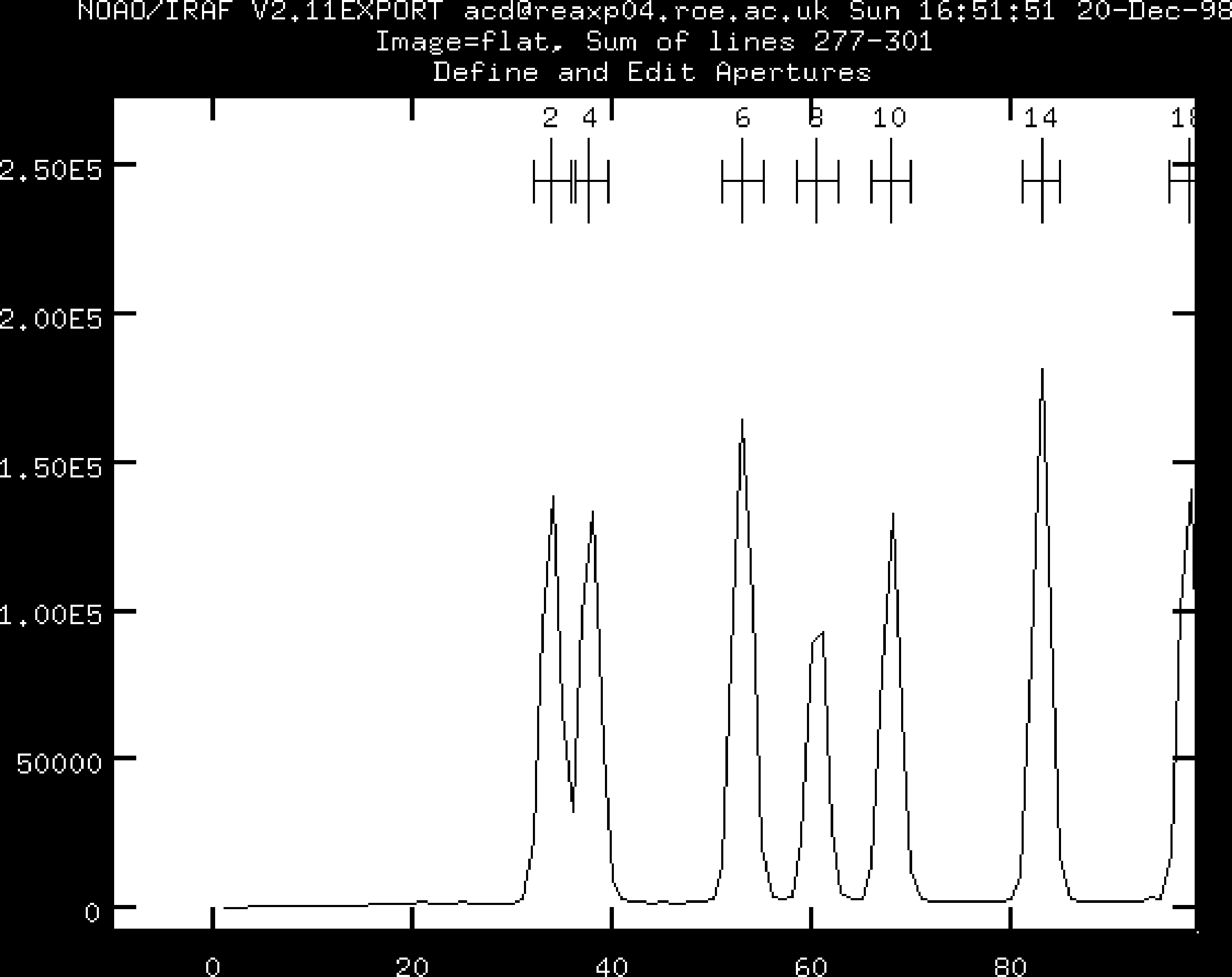
Reply yes to the prompts or just hit return. A plot similar to Figure 7 should appear. It shows a slice through the tramlines frame perpendicular to the dispersion direction. dofibers has attempted to identify the spectra but it will undoubtedly have made some mistakes which you will need to correct. You need to ensure that each genuine spectrum (object or sky) is correctly identified and no blanked off spectra are identified by mistake. You do this by comparing the identifications shown in the plot with the entries in the aperture identification file, apid.txt and changing the identifications in the plot until they agree with the file. The following points might be useful.

You interact with the plot by positioning the cursor and issuing one or two character commands from the keyboard. Help information about the commands available can be obtained by typing <shift>?, followed by hitting the space bar a few times to work through it and finally q to return to the interactive session. However, a few of the most useful commands are summarised below.

manipulating the plot
 
w j
resize the plot, setting the left edge at the current cursor position,
w k
resize the plot, setting the right at the current cursor position,
w t
resize the plot, setting the top at the current cursor position,
w b
resize the plot, setting the bottom at the current cursor position,
w a
resize the plot, auto-scaling it to show all the data,
r
redraw the plot.
renumbering spectra
 
d
delete the spectrum nearest to the cursor,
i
renumber the spectrum nearest to the cursor; you will be prompted to enter the new number,
q
quit.

Once you have finally got the numbered spectra to agree with the entries in the aperture identification file (which will take some time!) type q to quit this stage and proceed to the next.

(15)
Next dofibers traces the positions along the dispersion axis:
  Fit traced positions for flat interactively?  (yes);
  Fit curve to aperture 2 of flat interactively  (yes):


pdfpict
Figure 8: Trace along a FLAIR spectrum


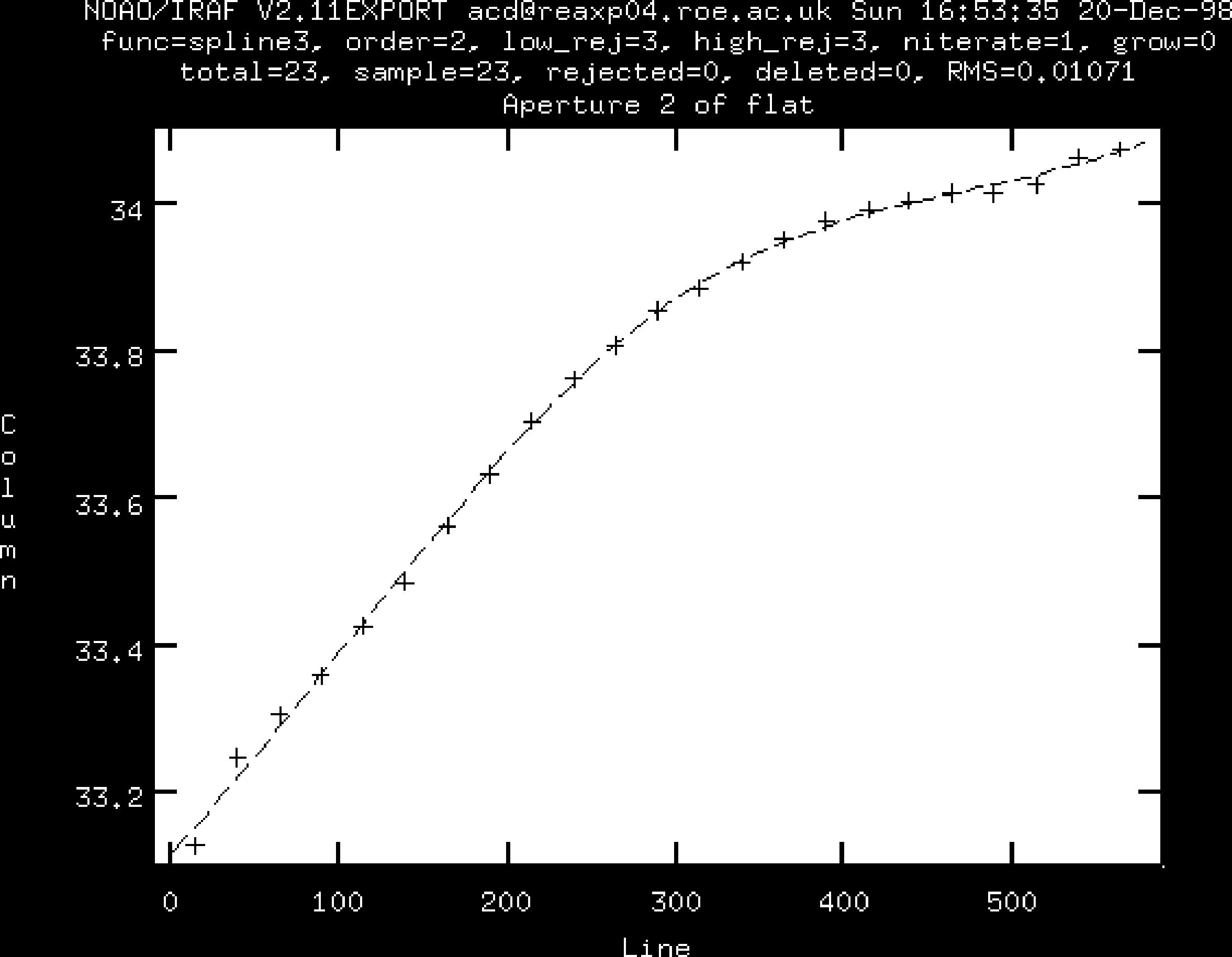
A plot similar to Figure 8 appears. For the example data you can simply accept the fit and type q and proceed to the next step. However, for other data you might want to edit the fit. dofibers then prompts:

  Fit curve to aperture 3 of flat interactively  (yes):

Reply NO (in upper case) so that the trace is applied to all subsequent spectra.

(16)
The next step is to wavelength-calibrate the spectra. The following messages appear:
  Create response function flatflatapid.t.ms
  Extract flat field flat
  Extract throughput image flat
  Correct flat field to throughput image
  Create the normalized response flatflatapid.t.ms
  Extract arc reference image arc
  Determine dispersion solution for arc

A plot similar to Figure 9 is drawn. You may need to adjust the plot limits to make your plot appear similar to Figure 9; use the plot manipulation commands given above. You need to identify the lines and enter their wavelengths. For the example data the wavelengths are marked on the plot. The example data contain unusually few lines, of which four are suitable for wavelength calibration. Using this small number of lines is conveniently simple for the example. However, the FLAIR arc lamps usually produce spectra with more lines and it is often desirable to have as many lines as practical in order to improve the calibration. FLAIR support staff should be able to advise about where to find suitable wavelengths. Proceed as follows.
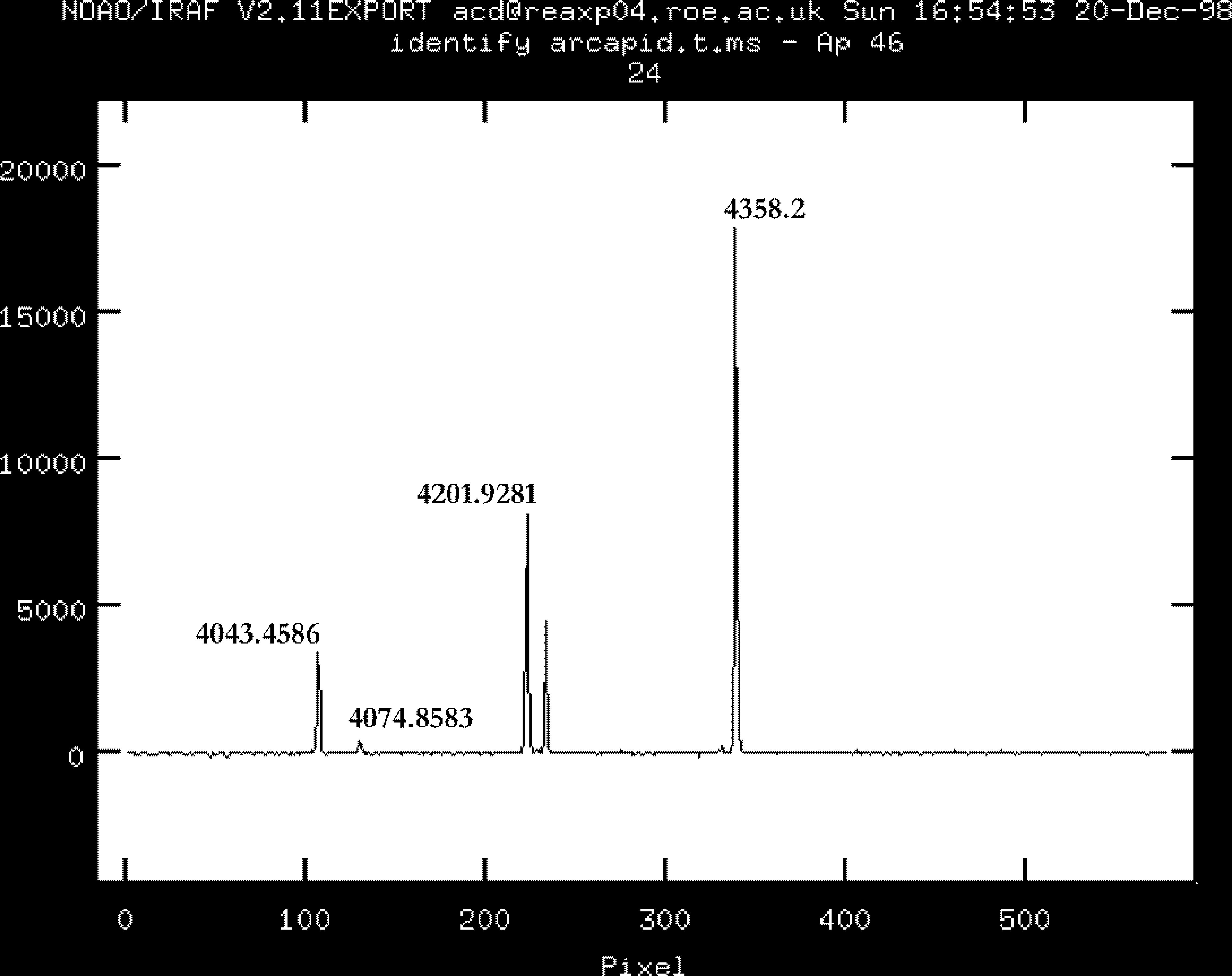

pdfpict
Figure 9: FLAIR line identification for wavelength calibration


(a)
Identify each line by placing the cursor over it and typing m. You will then be prompted to enter the appropriate wavelength in Å.
(b)
When you have identified all the lines type f to perform a fit.
(c)
By default a third-order fit is used. To change the order type :order followed by the required order. A second order fit is adequate for the example data. Type f again to re-fit the points with the new order.
(d)
Finally, when you are happy with the fit type q.

dofibers makes a preliminary wavelength calibration using the lines you have given, attempts to find further lines and displays all the additional lines it has found. You are then invited to inspect and amend these additional identifications. For the example data it is probably best to delete all the additional identifications. The useful commands are:

z
zoom on chosen line,
n
plot the next line,
d
delete line,
q
quit.


pdfpict
Figure 10: FLAIR sky spectra


You will then be prompted:

  Fit dispersion function interactively? (no|yes|NO|YES) (NO):

Reply NO. dofibers should display a list of line identifications and residuals:

  arcapid.t.ms - Ap 28    4/4     4/4       -1.08       -1.45  -3.5E-4 2.1E-11
  arcapid.t.ms - Ap 23    4/4     4/4       0.269       0.361  8.66E-5 8.0E-11
  arcapid.t.ms - Ap 10    3/4     3/3       0.963         1.3  3.09E-4 3.9E-12
  arcapid.t.ms - Ap 8     4/4     4/4       0.904        1.22  2.91E-4 3.8E-11
  arcapid.t.ms - Ap 32    4/4     4/4       -1.19       -1.61  -3.9E-4 1.2E-10
  arcapid.t.ms - Ap 88    4/4     4/4      -0.285      -0.383  -9.3E-5 1.3E-10
  arcapid.t.ms - Ap 90    4/4     4/4     -0.0497     -0.0663  -1.7E-5 4.0E-12
  arcapid.t.ms - Ap 91    4/4     4/4      -0.789       -1.06  -2.6E-4 2.3E-12
  arcapid.t.ms - Ap 92    4/4     4/4       -1.02       -1.37  -3.3E-4 6.7E-11
  Dispersion correct arc arcapid.t.ms: w1 = 3893.338768145233, w2 = 4729.910906658071, dw =
  1.323690092583605, nw = 633

and prompt:

  Change wavelength coordinate assignments? (yes|no|NO):

Again reply NO.

(17)
A further series of messages will appear:
  Extract object spectrum obj
  Assign arc spectra for obj
  Dispersion correct obj
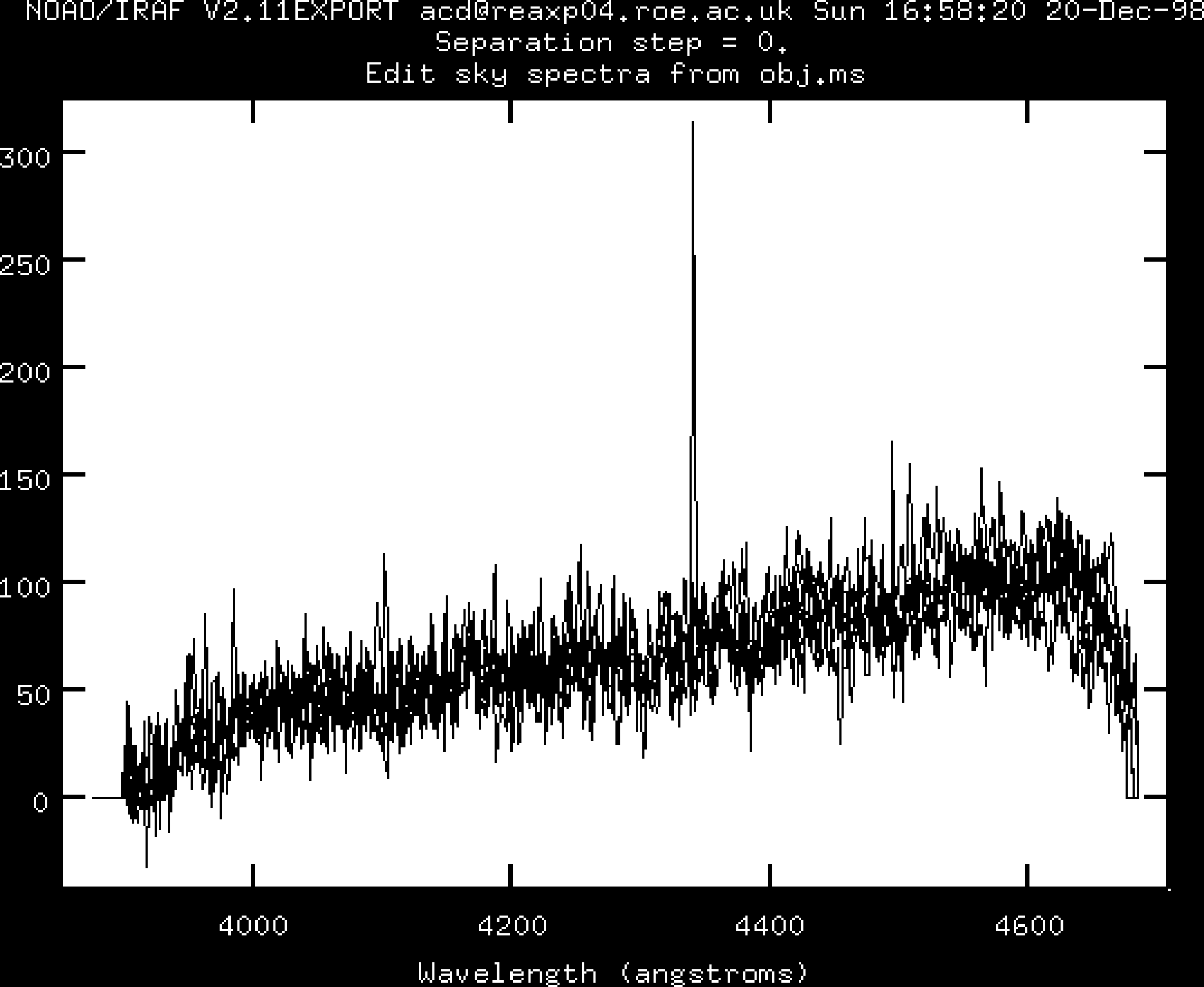
  Sky subtract obj:  skybeams=0
  Edit the sky spectra? (yes):

Reply yes and finally a plot of all the sky spectra will be drawn, similar to Figure 10. Again you may need to adjust the axes to reproduce the plot shown. You should delete any sky spectra which appear to deviate from the norm. In the example data no sky spectra need to be deleted. However, the procedure to delete a spectrum is to position the cursor over it and type d. Once you are happy with the remaining spectra type q to quit. You will be prompted for the technique to be used to combine the sky spectra:

  Sky rejection option (none|minmax|avsigclip) (none):

reply avsigclip. dofibers then terminates.

(18)
Sky-subtracted, wavelength-calibrated spectra have now been computed and are stored in IRAF image obj.ms (‘.ms’ for multiple spectra). To plot them type:
  splot  obj.ms

You will be prompted:

  Image line/aperture to plot (0:) (1):

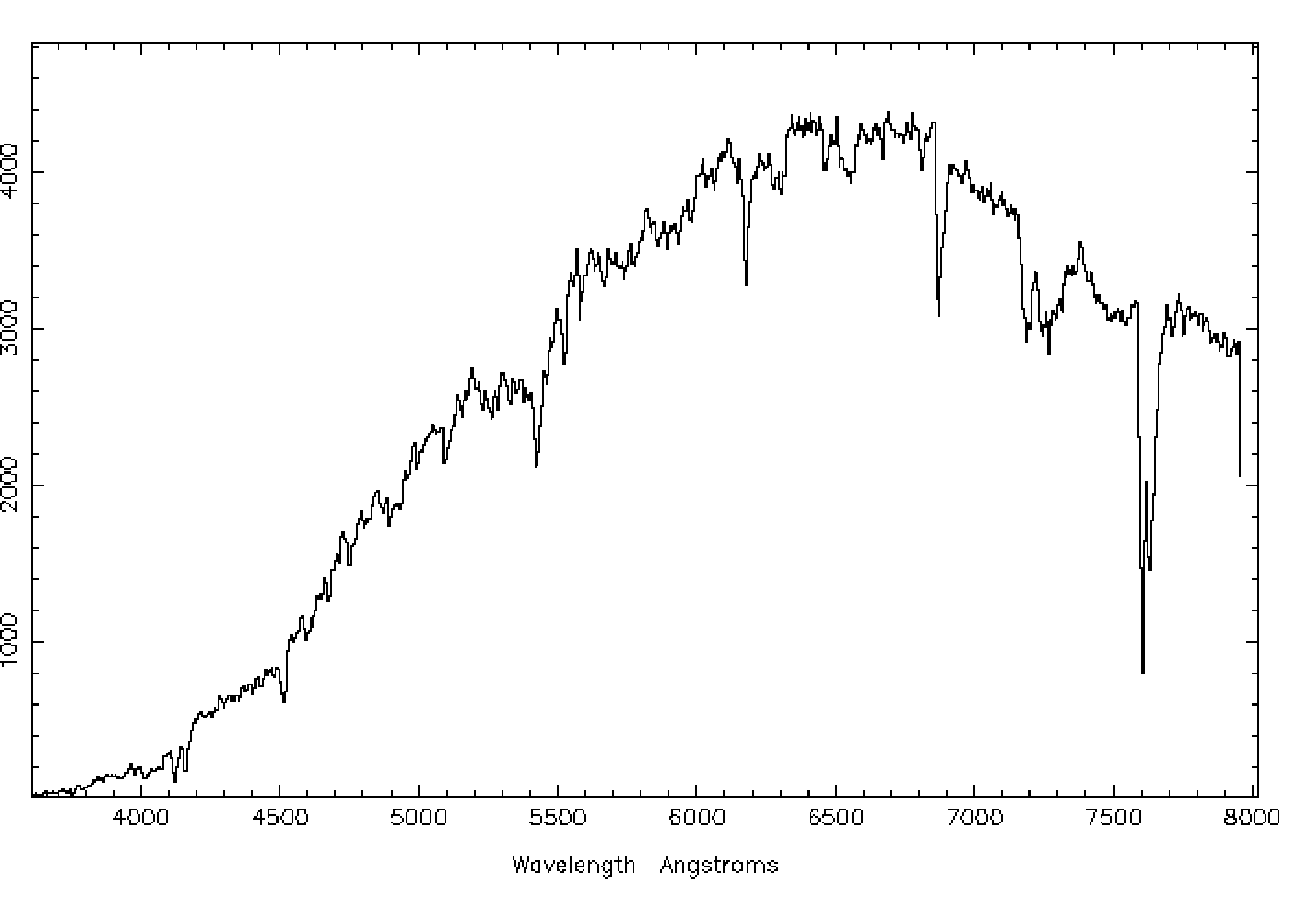
A plot similar to Figure 11 should appear. The axis ranges are adjusted in the usual way. Use ) and ( to step through the spectra (forwards and backwards respectively). When you have finished inspecting the spectra type q to quit.


pdfpict
Figure 11: FLAIR sky-subtracted, wavelength-calibrated object spectrum


12.1 Setup file customisation

The FLAIR setup script flairsetup.cl, is, of course, just a simple text file which can be listed or edited from the Unix shell. In order to use the file with your own data there are a couple of items which may need to be changed.

You should set the items combine.rdnoise and dofibers.readnoise to the readout noise of the CCD chip. The value can be obtained from the FLAIR Web pages.

You may also need to alter the extents of the bias and trim regions (ccdproc.biassec and ccdproc.trimsec respectively). If you are unsure about the appropriate values then the FLAIR support staff should be able to advise.

13 Reducing 2dF Data Using 2dFDR

This example demonstrates the use of the 2dFDR (2dF Data Reduction) package for reducing 2dF observations. 2dFDR was written at the AAO specifically for the reduction of 2dF data and it is the usual way to reduce these data. The example works through a complete simple reduction but nonetheless only shows a few of the features of the 2dFDR package. For a full description you should see the 2dF User Manual[3]. You need a colour display to use 2dFDR.

A sample dataset is available from the AAO and it is used in the present example. It is not included in the usual example directory for the present cookbook, but rather you should download it from the AAO along with 2dFDR (see below). The data comprises observations of galaxies with Bj<19.7 and quasars with Bj<21. They were acquired in January 1998 using 2dF plate 0 and spectrograph 1 and include arcs, flat fields, offset skys and target galaxy and quasar spectra. Though the observations are genuine the celestial coordinates have been randomised to preserve the proprietary rights of the original observers. The data are provided courtesy of the 2dF Bright Galaxy Survey and 2dF QSO Survey teams.

The procedure to use 2dFDR is as follows.

(1)
Obtain copies of 2dFDR and the example data from the AAO. See Section 7.1 for details. 2dFDR is available for the Digital/Alpha and Sun/Solaris versions of Unix. It requires some 25Mb of disk space (for the Digital/Alpha version) and the example data requires 40Mb. Both the software and example data are retrieved as compressed tar files. If you wish to have both the extracted files and the decompressed tar files resident on disk simultaneously then double the amount of disk space required.

All that is required to install 2dFDR is to simply extract the files from the tar archive. Similarly the example data are just extracted from the archive. For further details see file README included with each tar archive.

(2)
Prior to using 2dFDR you should set the environment variable DRCONTROL_DIR to the name of the directory where you have copied the files. For example, if I had put the files in directory /home/acd/2dfdr I would type:
  setenv  DRCONTROL_DIR  /home/acd/2dfdr

To set up for running 2dFDR type:

  source  $DRCONTROL_DIR/2dfdr_setup
(3)
2dFDR requires a large number of the colours on your display. Before starting it you should shut down any other applications which use many colours. Likely candidates are Netscape, SAOIMAGE or GAIA. If 2dFDR cannot obtain sufficient colours it will not start correctly.
(4)
Make the directory where you have copied the example data your current directory. Then type:
  drcontrol &

(The ‘&’ is, of course, simply to run drcontrol as a detached process.) A series of windows should appear.

(5)
Find the main window, which is called 2dF Data Reduction. It is shown in Figure 12.


pdfpict
Figure 12: 2dFDR main window


(6)
Click on the Commands menu (the rightmost of the three items in the menu bar in the top left of the window) and select the Find Fibres… option. A window similar to Figure 13 should appear. You need to select a file to be used to locate the position of the fibres. Click on file 29jan0033.sdf (which is a flat field and consequently suitable). Then click the OK button. A stream of processing information should be displayed in the terminal window from which you are running drcontrol and the main window.


pdfpict
Figure 13: 2dFDR window to choose the file to locate the fibre positions


(7)
A plot similar to Figure 14 should appear in the window labelled DRPLOT1 - Diagnostic Plots. 2dFDR should find all 200 fibres and their positions should match the overlays down the middle of the plot (ignore the edges at this point because the rotation is not yet fitted). Click on the Quit button in the DRPLOT1 - Diagnostic Plots window. File fibposa1.dat should be created in the example data directory.


pdfpict
Figure 14: 2dFDR initial fibre positions


(8)
Move back to the main window (Figure 12). Click on the Setup button (in the Auto Reduction box towards the top right of the window). The Setup Automatic Reduction window should appear, as shown in Figure 15. Simply click on the OK button. Further output should be displayed in the drcontrol terminal window.


pdfpict
Figure 15: Window to setup 2dFDR for automatic reduction


(9)
Again move back to the main window (Figure 12). Click on the Start button (in the Auto Reduction box). 2dFDR will process for a few minutes and a whole stream of output will be displayed in the drcontrol terminal window and the main window.
(10)
Still in the main window (Figure 12) click on the Commands menu again and this time choose the Combine Reduced Runs… option. A window similar to Figure 16 should appear. For the purposes of the example you should combine files 29jan0034.sdf, 29jan0035.sdf and 29jan0036.sdf. These files contain object frames and by combining them cosmic-ray events can be removed.


pdfpict
Figure 16: 2dFDR window to combine reduced runs


First click on file 29jan0034.sdf in the Files: box and then click on the >ADD> button. The file name (with a complete directory specification) should appear in the Files to be Combined box on the right hand side of the window. Repeat the procedure for files 29jan0035.sdf and 29jan0036.sdf. When you are finished the appearance of the window should be similar to Figure 16. If you add the wrong file by mistake then simply click on the REMOVE button. When you have assembled the correct list of files click on the OK button. Further output will be displayed in the drcontrol terminal window.

(11)
When the processing finishes the reduction is complete. Move to the main window (Figure 12) and close 2dFDR by clicking on the File menu (the leftmost item in the menu bar at the top of the screen) and choosing the Exit option.
(12)
The reduced spectra are stored in file combined_frames.sdf. This file is a two-dimensional array, with one axis corresponding to the fibre number (ranging from 1 to 200) and the other to wavelength.

The individual spectra can be plotted, for example, with Figaro (see SUN/86[43]). Type:

  figaro

To start Figaro. Then type:

  soft xw
  splot combined_frames\(,90\) autoscale=yes soft=xw

As is usual for Starlink software, the file name is specified without the .sdf file type. Also note how the backslash (‘’) is used to prevent the brackets being interpreted by the Unix shell (the use of Starlink applications from the Unix shell is discussed further in SC/4: C-shell Cookbook[15]). Simply hit return in response to the additional prompts from splot. Here spectrum number 90 is being displayed. A plot similar to Figure 17 should appear.


pdfpict
Figure 17: 2dFDR reduced galaxy spectrum


Acknowledgements

I am grateful to numerous people who contributed their time, expertise and data during the preparation of this cookbook. Nigel Hambly provided the data used in Section 12 and demonstrated the reduction of FLAIR data with IRAF. Dave Bowen provided the data used in Figures 3 and 4 and demonstrated the reduction of WYFFOS/AUTOFIB2 data with IRAF. Martin Clayton did much of the preliminary work on which the document is based. I had extremely useful discussions with Malcolm Currie and Quentin Parker. All the above and also Karl Glazebrook, Fred Watson, Don Pollacco, Jim Lewis, Harvey MacGillivray, Martin Bly and Rodney Warren-Smith either answered queries and/or provided useful comments on the draft version of the cookbook.

Any mistakes, of course, are my own.

Bibliography

[1]   J. Allington-Smith, P. Bettess, E. Chadwick, R. Content, R. Davies, G. Dodsworth, R. Haynes, D. Lee, I. Lewis, J. Webster, E. Atad, S. Beard, R. Bennett, M. Ellis, P. Hastings, P. Williams, T. Bond, D. Crampton, T. Davidge, M. Fletcher, B. Leckie, C. Morbey, R. Murowinski, S. Roberts, L. Saddlemyer, J. Sebesta, J. Stilburn and K. Szeto, 1997, in Kontizas et al. op. cit. ([28]), pp73-79.

[2]   S. Arribas, E. Mediavilla and F.G. Watson (eds), 1998, Fiber Optics in Astronomy III, Astronomical Society of the Pacific Conference Series, 152.

[3]   J.A. Bailey and K. Glazebrook, 1997, 2dF User Manual (Anglo-Australian Observatory: Sydney).

[4]   S.C. Barden (ed), 1988, Fiber Optics in Astronomy, Astronomical Society of the Pacific Conference Series, 3.

[5]   S.C. Barden (ed), 1995, Fiber Optics in Astronomical Applications, Proc. SPIE, 2476.

[6]   S.C. Barden 1998, in Arribas et al. op. cit. ([2]), pp14-19.

[7]   S.C. Barden, T. Armandroff, P. Massey, L. Groves, A.C. Rudeen, D. Vaughnn and G. Muller, 1993, in Gray op. cit. ([21]), pp185-202.

[8]   J. Barnes, 1993, A Beginner’s Guide to Using IRAF (National Optical Astronomy Observatories: Tucson). See SG/12 op. cit. ([34]) for details of obtaining IRAF manuals.

[9]   D.V. Bowen, M. Pettini and B.J. Boyle, 1998, Mon. Not. R. Astron. Soc, 297, pp239-250.

[10]   R.D. Cannon, 1997, in Kontizas et al. op. cit. ([28]), pp33-40.

[11]   J.W. Chamberlain, 1961, Physics of the Aurora and Airflow, International Geophysics Series, 2, (Academic Press: New York).

[12]   Y. Chu, 1997, in Kontizas et al. op. cit. ([28]), pp67-72.

[13]   M.J. Clayton, 1998, SC/7.2: Simple Spectroscopy Reductions (Starlink).

[14]   M.J. Currie and D.S. Berry, 1998, SUN/95.13: KAPPA – Kernel Application Package (Starlink).

[15]   M.J. Currie, 1998, SC/4.2: C-shell Cookbook (Starlink).

[16]   M.J. Currie, G.J. Privett, A.J. Chipperfield, D.S. Berry and A.C. Davenhall, 1998, SUN/55.10: CONVERT – A Format-conversion Package (Starlink).

[17]   A.C. Davenhall, 1998, SUN/190.6: CURSA – Catalogue and Table Manipulation Applications (Starlink).

[18]   A.C. Davenhall, G.J. Privett and M.B. Taylor, 1999, SC/5.2: The 2-D CCD Data Reduction Cookbook (Starlink).

[19]   P.W. Draper, 1998, SUN/139.9: CCDPACK – CCD Data Reduction Package (Starlink).

[20]   M. Drinkwater and B. Holman, 1996, FLAIR Data Reduction with IRAF (Anglo-Australian Observatory: Sydney).

[21]   P.M. Gray (ed), 1993, Fiber Optics in Astronomy II, Astronomical Society of the Pacific Conference Series, 37.

[22]   W.D. Heacox and P. Connes, 1992, Astron. Astrophys. Rev, 3, pp169-199.

[23]   J.Hecht, 1998, Understanding Fiber Optics, (Prentice Hall: Saddle River, New Jersey).

[24]   J.Hecht, 1999, City of Light, (Oxford University Press: Oxford).

[25]   J.M. Hill, 1988, in Barden op. cit. ([4]), pp77-92.

[26]   J.M. Hill, J.R.P. Angel, J.S. Scott, D. Lindley and P. Hintzen, 1980, Astrophys. J. Lett, 242, ppL69-L72.

[27]   D.C. Kay and J.R. Levine, 1995, Graphics File Formats, second edition
(Windcrest/McGraw-Hill: New York). See in particular Chapter 18, pp235-244.

[28]   E. Kontizas, M. Kontizas, D.H. Morgan and G.P. Vettolani (eds), 1997, Wide-Field Spectroscopy (Kluwer Academic Publishers: Dordrecht).

[29]   J.R. Lewis, 1996, WYFFOS Data Reduction Manual (Royal Greenwich Observatory: Cambridge).

[30]   C. Lissandrini, S. Cristiani and F. La Franca, 1994, Publ. Astron. Soc. Pacific, 106, pp1157-1164.

[31]   S.J. Maddox and A. Aragón-Salamanca (eds), 1995, Wide Field Spectroscopy and the Distant Universe, the 35th Herstmonceux Conference (World Scientific: Singapore).

[32]   P. Massey, 1997, A User’s Guide to CCD Reductions with IRAF (National Optical Astronomy Observatories: Tucson). See SG/12 op. cit. ([34]) for details of obtaining IRAF manuals.

[33]   P. Massey, F. Valdes and J. Barnes, 1992, A User’s Guide to Reducing Slit Spectra with IRAF (National Optical Astronomy Observatories: Tucson). See SG/12 op. cit. ([34]) for details of obtaining IRAF manuals.

[34]   R. Morris, G.J.  Privett and A.C. Davenhall, 1998, SG/12.1: IRAF – Image Reduction Analysis Facility (Starlink).

[35]   R. Morris and G.J.  Privett, 1966, SUN/166.4: SAOIMAGE – Astronomical Image Display (Starlink).

[36]   G.W. Nelson, 1988, in Barden op. cit. ([4]), pp2-22.

[37]   Q.A. Parker, 1997, in Kontizas et al. op. cit. ([28]), pp25-31.

[38]   Q.A. Parker and M. Hartley, 1997, in Kontizas et al. op. cit. ([28]), pp17-23.

[39]   Q.A. Parker, F.G. Watson and S. Miziarski, 1998, in Arribas et al. op. cit. ([2]), pp80-91.

[40]   I.R. Parry, 1997, in Kontizas et al. op. cit. ([28]), pp3-16.

[41]   I.R. Parry, 1998, in Arribas et al. op. cit. ([2]), pp3-13.

[42]   I.R. Parry and E. Carrasco, 1990, in Instrumentation in Astronomy VII, Proc. SPIE, 1235 pp702-708.

[43]   K.T. Shortridge, H. Meyerdierks, M.J. Currie, M.J. Clayton, J. Lockley, A.C. Charles, A.C. Davenhall and M.B. Taylor, 1998, SUN/86.16: FIGARO – A General Data Reduction System (Starlink).

[44]   F. Valdes, 1992, Guide to the Multifiber Reduction Task DOFIBERS (National Optical Astronomy Observatories: Tucson). See SG/12 op. cit. ([34]) for details of obtaining IRAF manuals.

[45]   F. Valdes, 1992, Guide to the Slit Spectra Reduction Task DOSLIT (National Optical Astronomy Observatories: Tucson). See SG/12 op. cit. ([34]) for details of obtaining IRAF manuals.

[46]   G. Walker, 1987, Astronomical Observations – An Optical Perspective (Cambridge University Press: Cambridge).

[47]   R.F. Warren-Smith, 1998, SUN/33.6: NDF – Routines for Accessing the Extensible N-Dimensional Data Format (Starlink).

[48]   F.G. Watson, 1995, in Maddox and Aragón-Salamanca op. cit. ([31]), pp25-32.

[49]   F.G. Watson, A.R. Offer, I.J. Lewis, J.A. Bailey and K. Glazebrook, 1998, in Arribas et al. op. cit. ([2]), pp50-59.

[50]   D.C. Wells, E.W. Greisen, and R.H. Harten, 1981, Astron. Astrophys. Suppl, 44, pp363-370.

[51]   F.G. Wyse and G. Gilmore, 1992, Mon. Not. R. Astron. Soc, 257, pp1-10.