A Data Characteristics and Issues

S2SRO data, due to our changing understanding of the instrument during shared risks observing, presents some particular challenges.

In order to illustrate in more detail some characteristics and issues associated with the SCUBA-2 data taken for the S2SRO, we will walk through an attempt to manually reduce a 850 $\mu$m observation on CRL 618 taken as observation 28 on 20100217.

A.1 Introduction data issues

There is no recommended procedure for manually reducing SCUBA-2 data, hence what follows is mainly intended to show the data issues rather than deliver a science product. Typically manual processing will remain inferior to the output of the iterative mapmaker. Note: a number of measures will be taken to address some of the issues seen during the S2SRO when upgrading SCUBA-2 to its full complement of 8 arrays. In particular in connection to the 30-sec fridge cycle, which dominates the common-mode signal, and a thermal gradient across the array that prevented the use of bolometers around the edge.

A listing of the observation directory shows the following:

As explained in the main section of the manual, the first and last files typically are ‘dark’ or ‘flatfield ramp’ observations. The remaining files can all be concatenated without resulting in too large a data set (which for science observations often will not be true unfortunately).

A.2 Telescope tracking

A first inspection can be made of the tracking of the telescope by inspecting the JCMT state structure in the headers:

Select a 2-D image panel and the columns x = TCS_TR_AC1, y = TCS_TR_AC2 to show the actual tracking on the sky. Each point marks the position of tracking center for each of the 200 Hz samples. By contrast the demanded tracking can be plotted using x = TCS_TR_DC1, y = TCS_TR_DC2. The resulting figures are shown in Fig. 18.

 

Figure 18: left: Actual tracking; Right: Demanded tracking

Obviously, for this observation the telescope failed to follow the demanded daisy pattern due to its acceleration limits. This failure to follow the demanded daisy pattern is often seen at higher elevations (this observation was at an elevation of approximately 72 deg). The demanded daisy is 120 arcsec across, i.e. even for the failed pattern a 3 arcmin field was almost always covered by the footprint of the bolometer array.

Hence, although in general not disastrous for compact daisy fields, the distribution of the tracking points may result in more systematics across the field. In particular the diagonal pattern can result in a ‘groove’ in the final image when using the standard configuration file in DIMM. Switching to dimmconfig_bright_compact.lis can help.

A.3 Flat field

Note: As explained in §B.3.2, observations taken after 20100223UT include a fast flatfield ramp at their start and end. Smurf will use these to calculate the flatfield dynamically. Earlier observations have a flatfield in their headers calculated by the online system from an explicit flatfield observation taken some time prior to the observation. These flatfields are less reliable due to the variability of flatfields and the observations should be treated with caution. It is recommended that flatfield and copyflat should be used to re-calculate and re-insert the flatfield using the, now default, better ramp-fitting techniques.

The above sc2concat command applies the flatfield to the data (it does so by default). Collapsing the time series of the concatenated and flatfielded file to calculate the mean signal for each bolometer results in Fig. 19 showing the bolometer map for the s8d array used during the S2SRO: a number of dead columns can be seen as well as regions around the perimeter where the thermal gradient caused problems biasing bolometers.

Figure 19: Mean signal in time-series

The range of the mean value in the map is very large: from $-$28 to 30. An inspection of the cube shows that much of this is caused by differing DC levels across the bolometers. The DC term can be removed using sc2clean (mfittrend can be used as well). In general, for relatively compact sources it should be safe to remove a first order baseline to also account for a monotonic drift component in the time series.

Collapsing the time-series cube again now results in a mean in a range of $-$3.0e-13 to 2.4e-13 as shown in Fig. 20. A histogram of the DC-removed data shows that the majority of the time-series data now are in a range of $-$0.1 to 0.1.

 

Figure 20: left: Mean signal in DC-removed time-series; Right: Histogram of values in DC-removed time series

A.4 Spikes and Steps

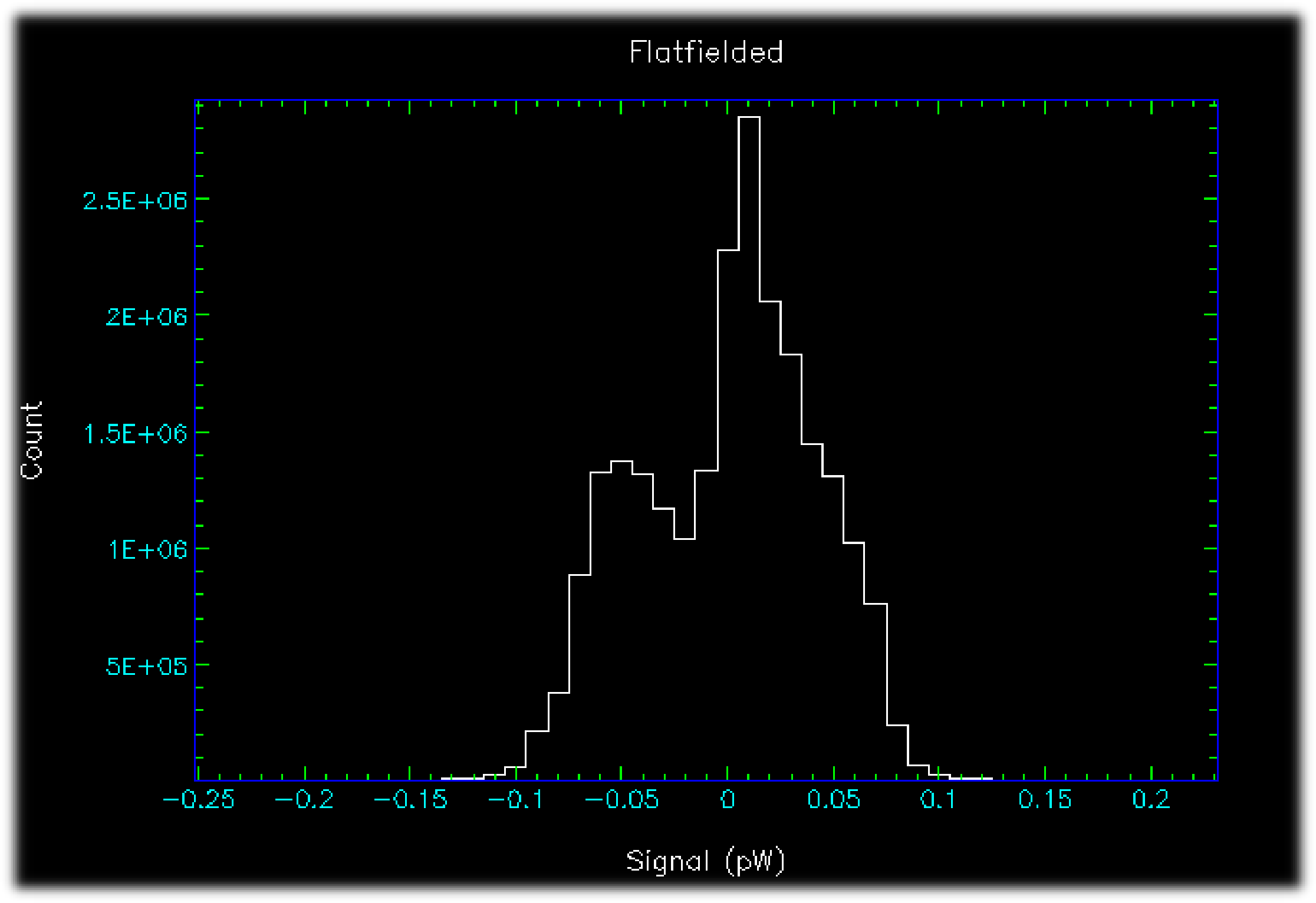
However, there are still significant outliers: the minimum and maximum pixel values are $\sim$8.1 and 3.4, respectively. Using Gaia to examine the time series in the DC-subtracted cube reveals remaining data issues as shown in the Fig. 21.

Figure 21: Example time series in the DC-corrected data set showing spikes, steps, and noisy bolometers. The dominant common-mode signal is a variation due to a 30 s temperature cycle in the dilution fridge. Top-left: a bolometer with a typical time series. Variations due to the 30 s fridge oscillation are obvious. Since all bolometers share this oscillation it is a ‘common-mode’ signal, but the amplitude may vary for different bolometers. Top-right: a bolometer with spikes in the time series. Middle-left: a bolometer with a moderate ‘step’. Steps can be introduced by the bias for that bolometer ‘rolling-over’ as it reaches its limit. During the S2SRO the instrument software that flags these events was not active. Middle-right: a bolometer with a large step. Bottom-left: a bolometer with multiple steps and spikes. Bottom-right: a ‘noisy’ bolometer.

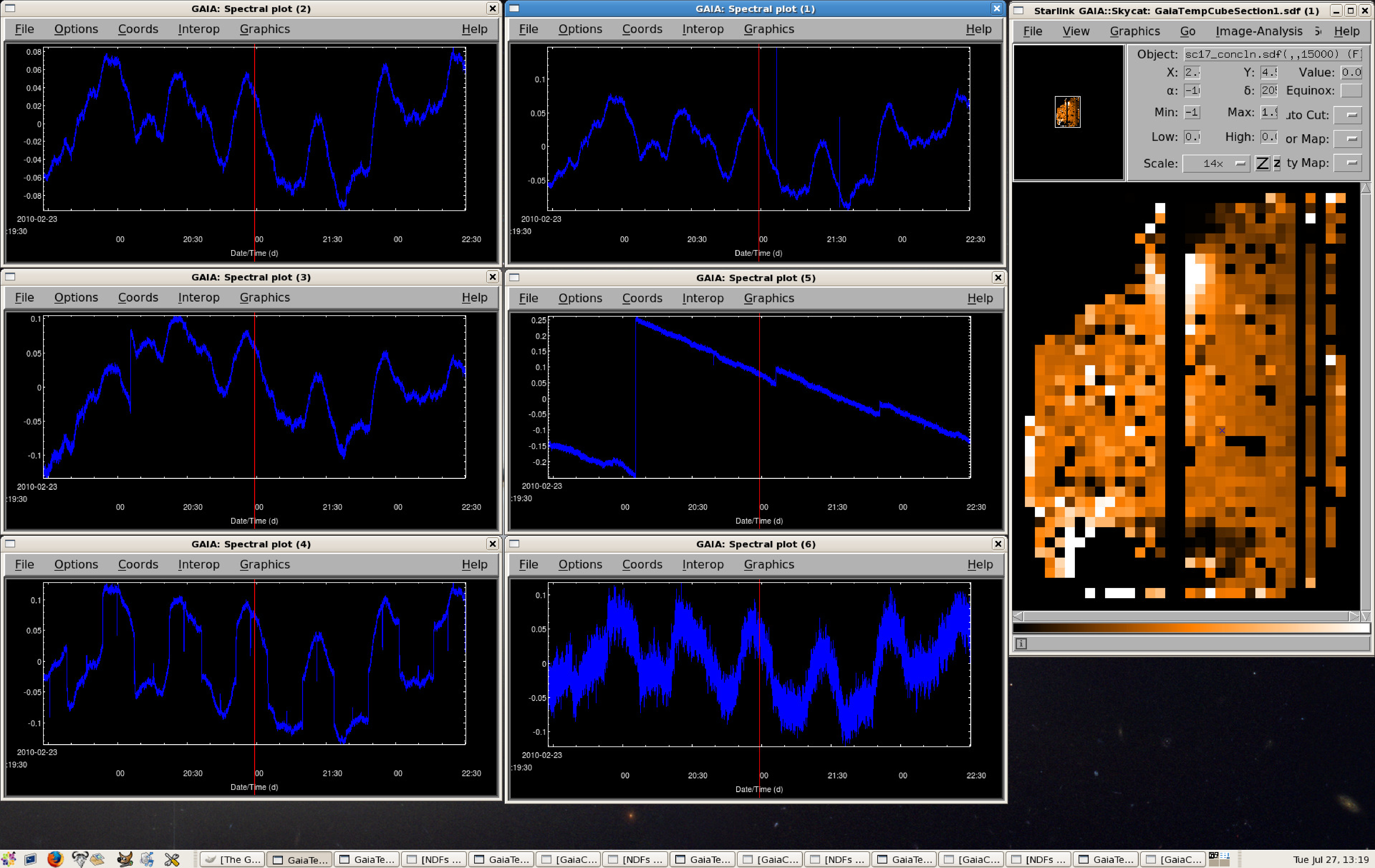
sc2clean is quite efficient in finding steps, but its spike removal is of limited effectiveness in the presence of a strong common-mode signal. As an example sc2clean was re-run with the following configuration file:⁸

The results were that sc2clean left the time series of the top two plots in Fig. 21 unchanged, i.e. the common-mode variation was too large to cause the spikes in the right time series to be flagged. sc2clean completely flagged the two time series on the bottom row as bad. It did an excellent job correcting for the steps in the middle row time series, as shown in Fig. 22.

 

Figure 22: Original (white) and sc2clean step-corrected (red) time series.

A.5 Common Mode Signal

To investigate features of the time series further one needs to get rid of the dominant common-mode signal. Most of the variation seen is due to a 30-sec temperature cycle of the dilution fridge. This cycle affects the biasing of the bolometers and, in effect, varies the zero-level of each on that time-scale. There are various ways to remove this signal for quick inspection of the data, but here are two. Again, please be reminded that the aim here is not to reduce the data for map-making, but to illustrate characteristics of the data set.

Method 1: The simplest method is to mimic the action of the SMO module of the DIMM: subtract the median in a sliding box from the time series.

Method 2: Use the DIMM to subtract the common-mode signal and export the models for further inspection. The common-mode is captured by the COM, GAI, and FLT models as GAI*COM+FLT.

A.5.1 Method 1

The first method can be implemented rather simply using ‘block’ although the calculation of the sliding medians will take quite long. Since the time series corresponds to a path across the sky, this obviously suppresses any structures larger than the path corresponding to the box. However, it is a very efficient method to flatten the time series (including steps which can change into spikes) to allow an easy statistical analysis of the intrinsic noise characteristics of bolometers. This ‘harsh selection’ method may have merits for the analysis of point-source fields, but be aware that the DIMM in general will leave significantly more ‘baseline’ systematics in the time-series.

A block-size of 200 corresponds to 1 sec of data, which can be related to a spatial size through the maximum scanning speed e.g. 120 arcsec/sec. Remember though that the telescope spends a large fraction of the time at lower speeds either accelerating or decelerating. In fact, a block-size of 200 largely removed the signal from CRL 618 from this data set!

Figure 23: Example time series in the block-median common-mode subtracted data set high-lighting intrinsic noise issues that can be seen in bolometers. The top-left time series is the same as the top-left time series in figure Fig. 21

An inspection of resulting file shows very flat time series. The top-left panel in the Fig. 23 shows a typical time-series after removal of a sliding median. The next two panel show time-series with negative and positive spikes. The middle-right panel shows a bolometer with an increased noise during part of the scan. The next two panels show bolometers with an uneven noise performance. Note that the DIMM will not specifically handle these issues, apart from de-spiking and an iterative clip of bolometers based on their overall noise level. It also is the case the residual variations remaining after a common-mode subtraction often are of a similar or larger level: the sliding-median method allows one to zoom in on the noise characteristics of individual bolometers and possibly derive a bad-bolometer map for use with the DIMM (many SCUBA-2 tasks accept a ‘bbm’).

A word of caution: at the high scanning speeds, point-like sources will look as spikes in the time series. At 120 arcsec/sec it takes the telescope at least 10 samples to cross the 45 $\mu$m beam. However, at 600 arcsec/sec (as may be used for large scan maps), the crossing happens in barely more than 2 samples!

One can attempt to further identify problematic bolometers by, for example, calculating the rms of each time series, but that falls outside the scope of this document:

A.5.2 Method 2

Method 2 is to use the DIMM to derive the common mode signal. The common-mode signal will be GAI*COM+FLT. There are a few gotchas to keep in mind though (note that some of these may change as the program gets further optimized):

• The DIMM will do a sc2clean in a preprocessing step which makes it hard to compare the models to the original file. At the least do an external DC removal first (as outlined above). Or do the sc2clean as an external step and switch off all sc2clean parameters in the dimmconfig file submitted to the DIMM.
• The DIMM will add padding on either side of the time series but not remove it from the models before writing them out. There currently is a bug that requires one to use ‘setorigin’ to properly align these cubes with the original one.
• The current FLT model will apodize (i.e. smoothly reduce the ends of the time series to zero; these ends are not used for the mapmaking). The apodization is needed for FLT’s current FFT, but a non-apodizing FFT method is under development.
• com.notfirst regulates whether the COM model is run during the first iteration. If set to 1, most of the dominant fridge-related variations will end up in the FLT model. A priori this is not a problem as far as removing the signal is concerned, but the FLT model works on each time series individually i.e. does not really derive a common-mode.
• Related to the previous point, if the fridge variations end up in the FLT model, the GAI model will not really show the gain variation across the bolometers, since the COM model in that case will only contain the residual common-mode variation (often dominated by ringing artefacts from FLT’s FFT). i.e. for this exercise we want to make sure that com.notfirst=0.
• The first plane of the GAI model has the multiplicative term but it is distributed around the median (or mean) gain rather than a value of 1 due to the way that the GAI and COM models have been implemented. i.e. divide the gain map by its median in order to get a value distributed around 1. However, note a subtlety: the gain of each bolometer in principle should have been fitted and accounted for by the flat field. Any gain differing from 1 in the GAI model can be interpreted as either a poor flat-field fit, the gain being variable, or some basic bolometers characteristics, e.g. their individual resistances, not (yet) being accounted for sufficiently.

For example, for these observations of CRL 618 modify the dimmconfig_bright_compact.lis configuration file as follows. Given that, at the time of writing, the FLT model apodizes, it has been left out.

A reminder: this exercise aims at showing data features and not at showing how well the DIMM can handle these. For the latter one would want to run the DIMM with all its features enabled.

The above file exports all relevant models. It produces a moderately smoothed common mode time series and a single gain component for the whole observation. A script that handles combines the output models into a common-mode and common-mode subtracted cube is appended at the end of the document. It actually gives us three useful files to look at: the derived common-mode signal (_commode), the relative gains of the bolometers (_gain), as well as a common-mode subtracted cube (_astres).

Figure 24: Example time series (white) and the derived common-mode signal (red). This time series is the same as the top-left time serie in Figs. 21 and 23

Fig. 24 shows a typical time series with the fitted common-mode signal.

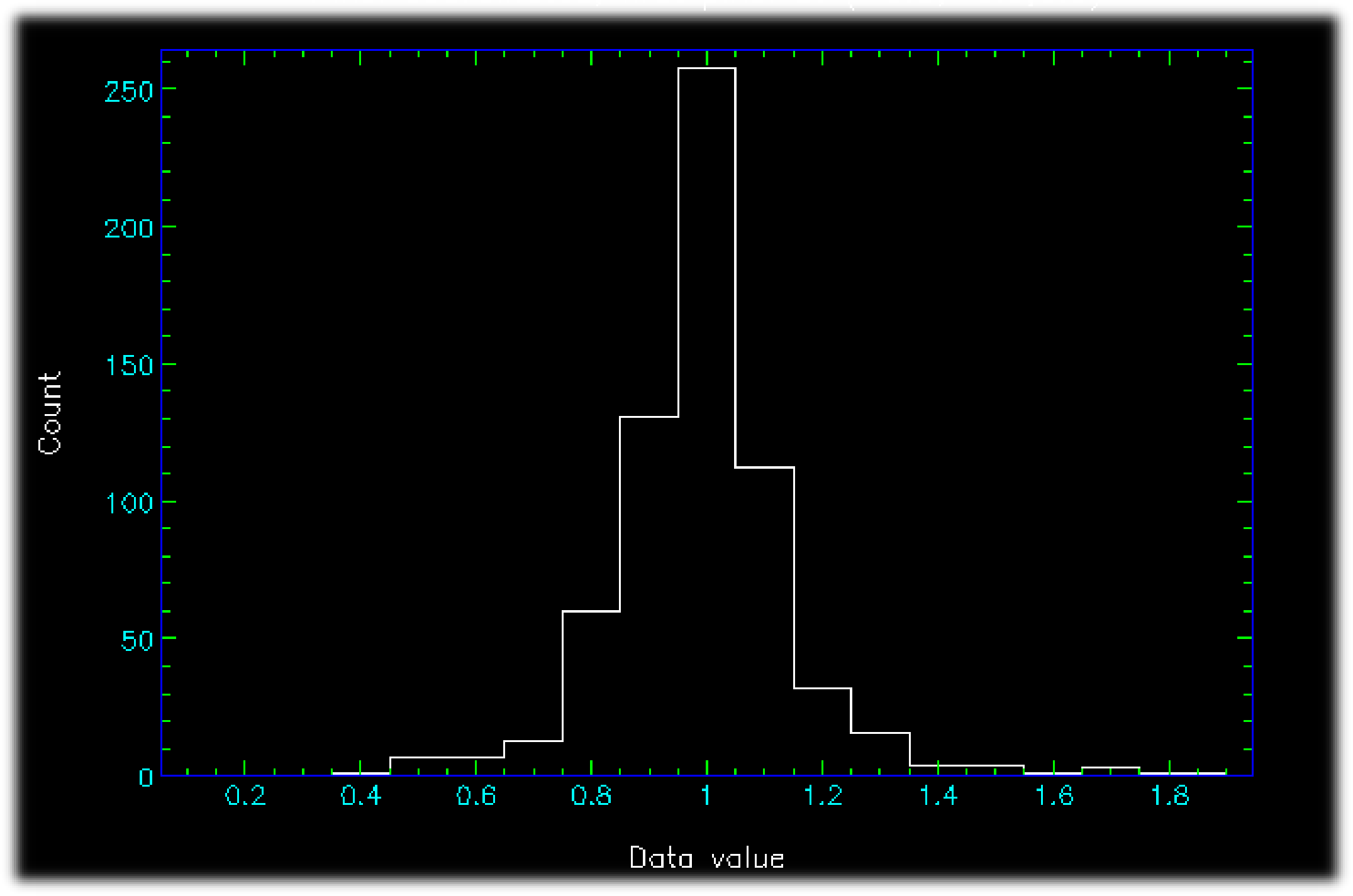
The input cube to makemap had 812 ‘good’ bolometers, the derived gain map 651: makemap has flagged an additional 161 bolometers as bad. A quick inspection of the masked bolometers shows that the majority have steps, increased noise, or multiple spikes. The gain map itself ranges from 0.44 to 1.89 and a histogram shows that of the 651 unflagged bolometers 593 ($\sim$90 per cent) are within a range of [0.75,1.25] and 622 within [0.65,1.35]. To some degree this range indicates that for the S2SRO data the flat field in practice was in general not very accurate or stable probably due to one or more of the aforementioned reasons.

Figure 25: Histogram of the bolometer gains as derived by the DIMM based on their response to the common-mode signal. Note that these gains are, by default, only used for the subtraction of the common mode and not for the subsequent gridding into a map.

For a further analysis one can also e.g. collapse the common-mode subtracted cube over the time-series to calculate the median and rms:

The median signal ranges from $-$33e-04 to 30e-04, with 582 bolometers falling within a range of $-$5e-04 to 5e-04. The median rms is 3e-03 with a maximum of 14e-03 and 578 bolometers below a rms of 6e-03 (twice the median). The three panels in Fig. 26 summarize this information.

   

Figure 26: Left: Gain image: black $<$ 0.75, white $>$ 1.25; Middle: Common-mode subtracted median: black $<-$5e-04, white $>$ 5e-04 Right: Common-mode subtracted rms: white $>$ 6e-03 (twice the median).

The three maps have a significant subset of ‘flagged’ bolometers in common. An inspection of the common-mode subtracted data (_astres) shows that many of these bolometers have (multiple) steps that were not removed by sc2clean. Another subset shows variations that don’t seem well modeled by the common-mode signal, although one has be careful not to mark the signature from CRL 618 as bad. But even for bolometers that pass through all the selection ‘filters’ there are quite a few that still have spikes, steps, or baseline ripples. Although the mapmaker was deliberately crippled for the above presentation, further development of the mapping algorithms will be needed to optimally handle SCUBA-2 data and produce the best possible maps.

   

Figure 27: Sample time-series with a simple common-mode subtracted.

A.6 Maps

Although somewhat outside the scope of this document, after all this one might wonder what the maps from the various techniques looks like. Bear in mind that both a manual reduction as well as the mapmaker can be optimized better than is presented here. Apart from the first map, all the maps in Fig. 28 are presented with the same grey-scale stretch and show a 180 $\times$ 180 arcsec region around CRL 618.

   

Figure 28: Top left: Map of the concatenated data; Top right: After removing a linear baseline from the time series; Bottom left: After linear baseline, steps, and spike removal; Bottom right: Iterative map maker with dimmconfig_bright_compact.lis

A.7 Sample Common-mode script