Appendix F
Viewing your Data with KAPPA

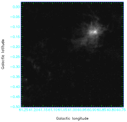
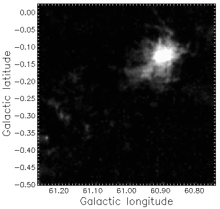
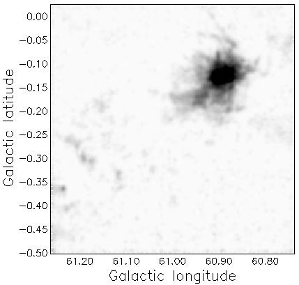
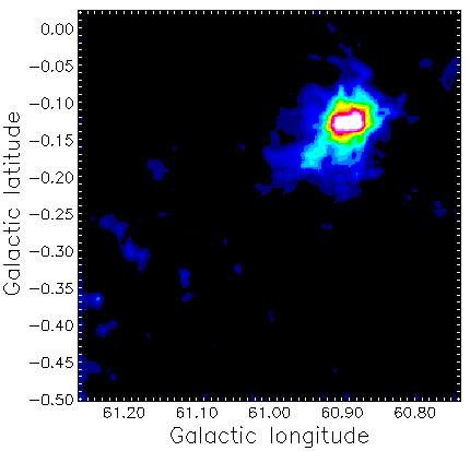
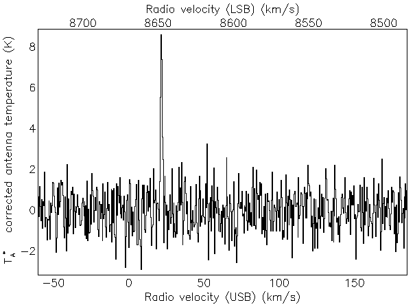
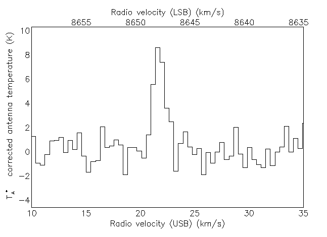
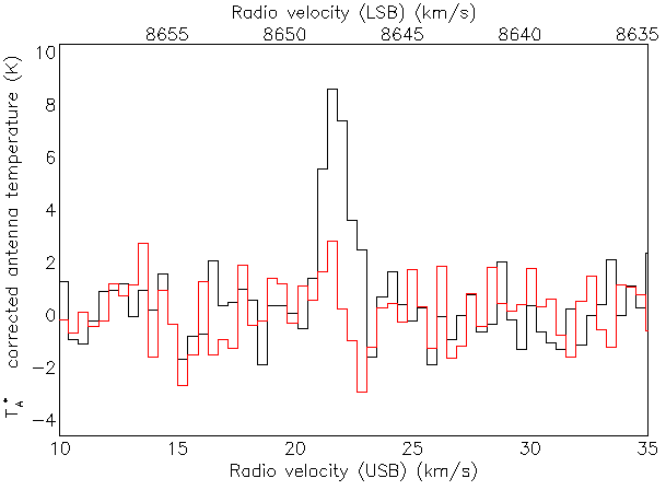
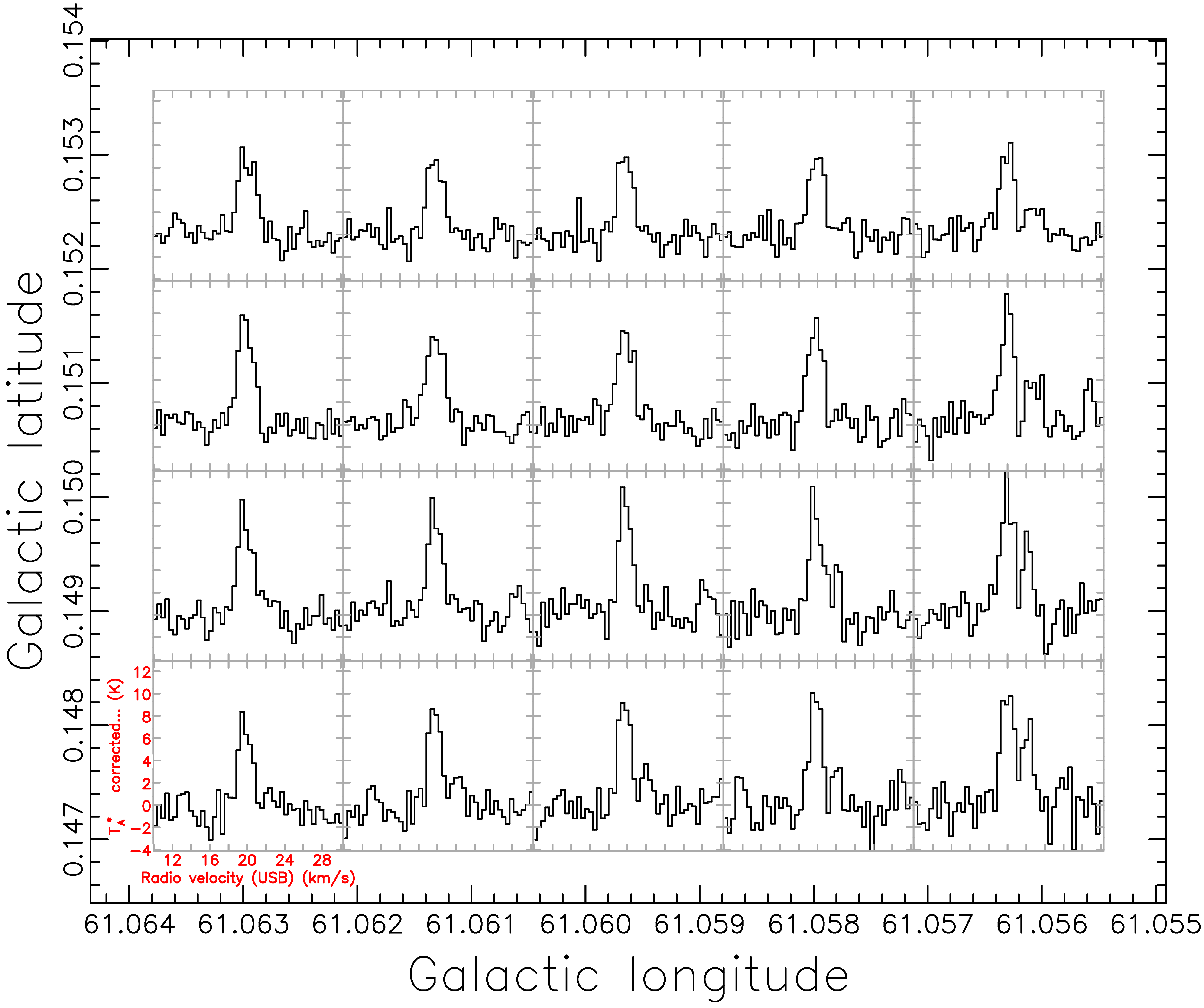
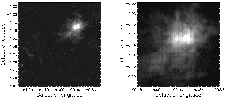
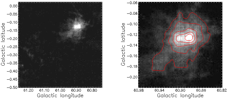
This appendix offers a few examples of creating different types of plots using Kappa. The applications highlighted here are display and contour for maps, and linplot and clinplot for spectra (See the Kappa manual for more details).

The plotting attributes for each of these applications is controlled in the same way. For full details of all the formatting options as well as setting up your graphics device, see the ‘Plotting Styles and Attributes’ section in the Kappa manual.

F.1 Setting up xwindows

• Clear my graphics window and reset default values.
    % gdclear
• Set my display device to xwindows.
    % gdset xw
• Create an xwindow of the desired dimensions.
    % xmake -width 1500 -height 1000 xwindows
• To create a display window which plots black on a white background, change the order of black and white in the palette list for your graphics device. Check this using gdstate.
    % gdstate

  Ensure white is entry 0 and black in entry 1.

    % palentry 0 White
    % palentry 1 Black

F.2 Format axes

• Use wcsattrib to set how your axes should be formatted. Here the format of the first and second axes is set to two decimal places for Galactic co-ordinates. Find out more about the Format attribute under wcsattrib in the Kappa manual.
    % wcsattrib map set format"(1)" .2
    % wcsattrib map set format"(2)" .2
• For FK5 co-ordinates you can use the same method to set exactly how the co-ordinates should be displayed. The example below sets R.A. units to $0^{h}00^{m}00^s$ and Dec. units to $00^{\prime }00^{″}$.
    % wcsattrib fk5map set format"(1)" ghms
    % wcsattrib fk5map set format"(2)" gdms

F.3 Plotting a two-dimensional image

• Display map.sdf. Do draw axes and a border, but do not draw a title or a grid. The default cut parameters for mode=scale include all the data.
    % display map border axes style=’"drawtitle=0,grid=0"’ mode=scale

  Depending on your default settings you may get a map like the one below.

  ---

  
  

  Figure F.1: First attempt at displaying an integrated map with Kappa:display.

  ---

• Re-draw calling a style file and changing the scaling.
    % display integ.sdf axes style=^style.dat mode=scale low=0 high=100

  ---

  
  

  Figure F.2: Displaying an integrated map with Kappa:display using a style file to format the plotting attributes.

  ---

  Below is a copy of the style file (style.dat) used to make Figure F.2.

    border=1
    tickall=1
    majticklen=0.01
    drawtitle=0
    color(axis)=white
    color(numlab)=black
    color(border)=black
    color(ticks)=white
    size(numlab)=1
    size(textlab)=1.5
    nogrid=1
    textlabgap(1)=0.01
    textlabgap(2)=0.01
• Make the colour scale negative and then replot.
    % lutneg
    % display integ.sdf axes style=^style.dat mode=scale low=0 high=100

  ---

  
  

  Figure F.3: Reversing the colour scale in Kappa:display.

  ---

• There are a number of colour palettes available in Starlink. You can find them in the $STARLINK_DIR//bin/kappa/ directory.
    % ls $STARLINK_DIR/bin/kappa/*lut.sdf

  You can create your own colour scheme using the Kappa routine lutedit. See the Kappa manual for more details.

• Replot in colour by selecting one of these palettes via the lut option.
    % display integ.sdf axes style=^style.dat mode=scale low=0 high=100 \
      lut=$STARLINK_DIR/bin/kappa/random3_lut

  ---

  
  

  Figure F.4: Displaying an integrated map in colour with Kappa:display.

  ---

F.4 Plotting spectra

• Plot the spectrum from cube.sdf at the position $l$=60.°87, $b$=0.°18. Use existing style.dat except override the text label size which is too big for these axes labels.
    % linplot "cube(60.87,0.18,)" style="’^style.dat,size(textlab)=1’"

  ---

  
  

  Figure F.5: Displaying a spectrum with Kappa:linplot.

  ---

• Re-plot, but this time only show the velocity range 10 to 35 km s$-1$. You can do it this way:
    % linplot "cube(60.87,0.18,-10:50)"  style="’^style.dat,size(textlab)=1’" \
      mode=histogram

  or using xleft and xright.

    % linplot "cube(60.87,0.18,10:35)"  style="’^style.dat,size(textlab)=1’" \
      mode=histogram xleft=10 xright=35 lmode=’"Extend,15,15"’

  In the example above, the additional option lmode is included. This sets how the upper and lower limits for the y-axis are defined. This example expands the minimum and maximum values by 15% of the data range. In additional extended, the available options are range, percentile and sigma.

  ---

  
  

  Figure F.6: Displaying a zoomed-in spectrum with Kappa:linplot.

  ---

• To plot a second spectrum over this one, re-call linplot but with the noclear option to keep the original plot underneath. The formatting defaults to the last time linplot was run, but with the one-off temporary change of setting the colour of the line to red. The plus sign means the change will not be remembered next time linplot is run.
    % linplot "cube2(60.87,0.18,-10:50)" mode=hist style="+colour(line)=red" \
      noclear

Figure F.7: Displaying two super-imposed spectra with Kappa:linplot.

F.5 Plotting a grid of spectra

• To plot multiple spectra from a cube you can use clinplot.
    % clinplot "cube(61.06~5,0.15~4,10.:30.)" nokey style=^style.dat reflabel \
      specstyle="’colour(textlab)=red,colour(numlab)=red’" mode=hist

  This example plots a grid of 5$\times$4 pixels around $l$=61.°06 and $b$=0.°15. Each spectrum has a range of 10 to 30 km s$-1$. Note the decimal points are necessary for the spectral limits, otherwise the spectrum would extend from pixel co-ordinates 10 to 30. The specstyle option allows you to format the spectral axes inside the main plot. The formatting options are the usual plotting attributes. The flag reflabel annotates the interior spectral axes.

Figure F.8: Displaying a grid of spectra with clinplot.

F.6 Plotting two images side by side

• Create a 2$\times$1 grid of frames.
    % picgrid 2 1
• Select the first frame.
    % picsel 1
• Display integ.sdf in the first frame.
    % display integ axes style=^style.dat mode=scale low=0 high=100
• Select the second frame.
    % picsel 2
• Display subinteg.sdf, a cut-out of integ.sdf, in the second frame.
    % display subinteg axes style=^style.dat mode=scale low=0 high=100

  ---

  
  

  Figure F.9: Displaying an image and a magnified portion of that image with Kappa:display.

  ---

• Still in the second frame, plot contours over the map from a smoothed version of subinteg.sdf.
    % contour smoothsub.sdf noaxes noclear nokey ncont=5 mode=free \
      heights="[40,80,120,160,200]" pens=’"width=3.0,colour=red"’

  ---

  
  

  Figure F.10: Displaying an image and a magnified portion of that image overlaid with smooth contours created with Kappa:display and contour.

  ---

F.7 Selecting a different graphics device

• You can view all available graphics devices with gdnames.
    % gdnames
• Instead of using gdset to define a new graphics device for all your applications, you can add the device option to select a different one for just this command. In the example below the output goes to a PostScript file called myplot.ps. The option pscol_l specifies landscape mode with colour. Setting a name for your output PostScript file is optional; if left unset it will default to pgplot.ps.
    % linplot "cube(60.85,0.18,-10:50)" mode=hist device="pscol_l;myplot.ps"
• If you want to combine the results of several applications into a single plot, you need to specify an encapsulated PostScript device, e.g. epsf_l. Once you have run all the application you can stack your list of PostScript files to produce a single file.
    % psmerge plot*.ps > final.ps