Processing math: 100%
Chapter 11
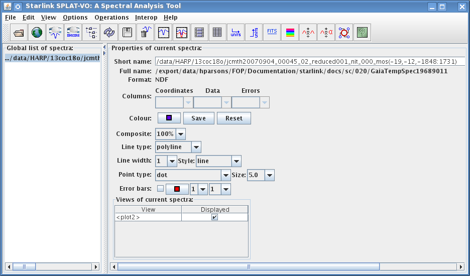
Using SPLAT
Splat is a graphical spectral-analysis tool. Splat offers tools for further processing, fitting, or identification of
spectral lines. One can also plot different spectra in the same window and make publishable files. The full
Splat documentation can be found in SUN/243.
11.1 Opening a spectrum in SPLAT
There are two options for opening up a spectrum in Splat. First it is possible to send a spectrum to Splat using
Gaia as described in Section 10.8.
Alternatively spectra can be displayed in directly in Splat using:
for a single position cube or
% splat ’filename(xpos,ypos,)’ &
to display the spectrum at the pixel position (xpos,ypos). Or simply initialise Splat and open the file directly
from the gui.
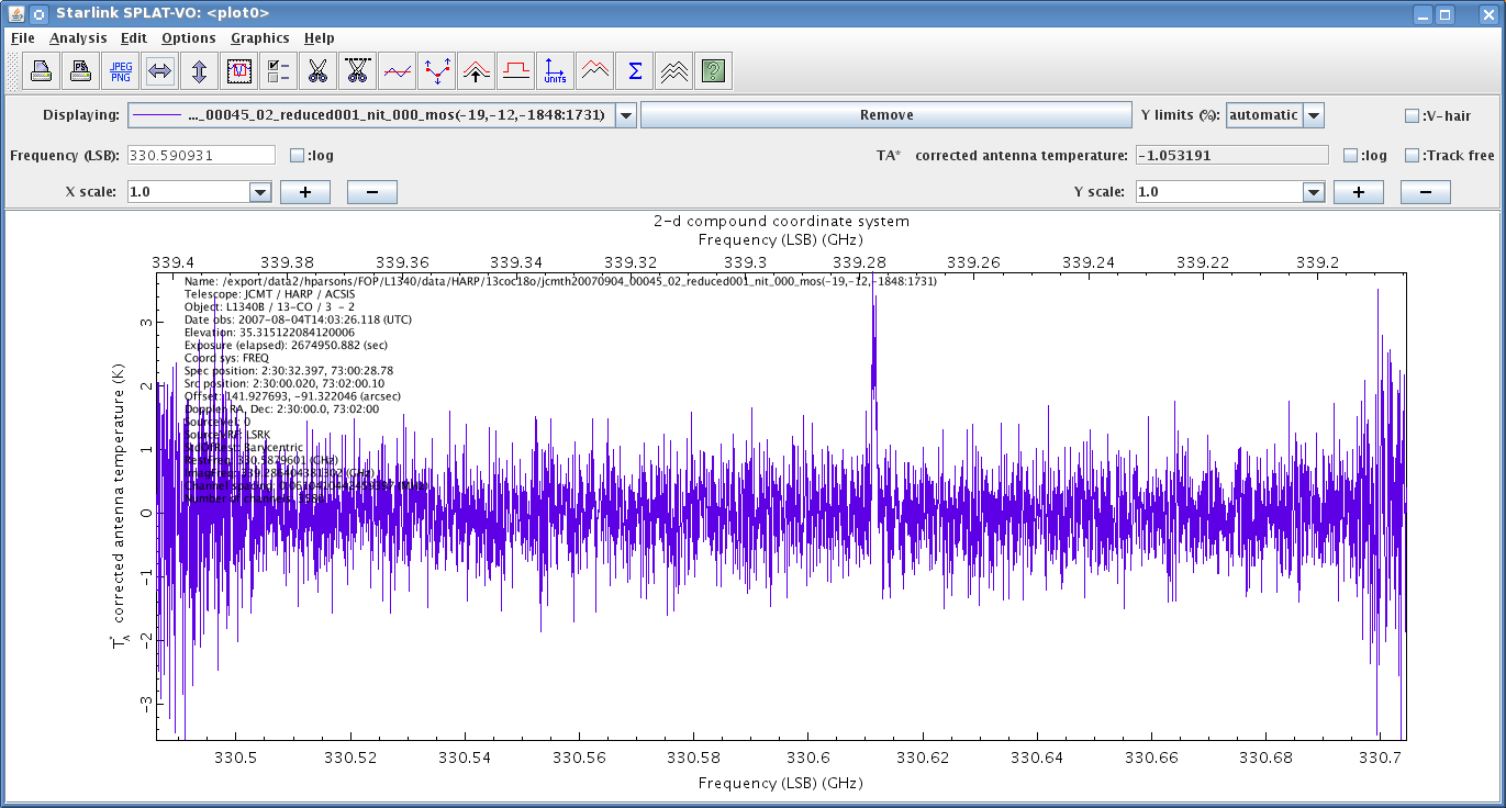
When Splat is initially started you will get a main window appear and also a spectral window.
11.2 Display synopsis of spectrum
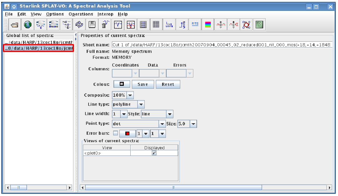
When you initially open a specrum in Splat the synopsis of that spectrum will automatically be overlaid on the
spectrum displayed, if the metadata are known to Splat. The following are a list of possible properties than can
be displayed, with a brief description. Names in parenthesis are either the FITS keywords or AST attributes
used to obtain the values.
-
(1)
- Name: the short name
-
(2)
- Telescope: telescope, instrument and its backend (
TELESCOP/INSTRUME/BACKEND)
-
(3)
- Object: target, molecule and molecular transition being observed (
OBJECT/MOLECULE/TRANSITI)
-
(4)
- Date obs: date of the observation (
DATE-OBS or Epoch in UTC)
-
(5)
- Elevation: observatory elevation (
ELSTART or 0.5∗(ELSTART+ELEND))
-
(6)
- Exposure: exposure time for the spectrum (
EXTIME)
-
(7)
- Exposure (median): exposure time for the spectrum (
EXP_TIME)
-
(8)
- Exposure (elapsed): the time elapsed during exposure (
INT_TIME otherwise DATE-END−
DATE-OBS)
-
(9)
- Exposure (effective): effective exposure time (
EXEFFT)
-
(10)
- Coords sys: the co-ordinate system code (System)
-
(11)
- Spec position: position of spectrum on the sky (
EXRAX, EXDECX)
-
(12)
- Src position: position of the observation centre (
EXRRA, EXRDEC)
-
(13)
- Img centre: centre of the originating image (
EXRA, EXDEC)
-
(14)
- Offset: offset of spectrum from the observation centre (
EXRRAOF, EXRDECOF or EXRAOF, EXDECOF)
-
(15)
- Doppler RA Dec: reference position (RefRA,RefDec)
-
(16)
- SourceVel: source velocity (SourceVel)
-
(17)
- SourceVRF: source velocity reference frame (SourceVRF)
-
(18)
- SourceSys: system of the source velocity (SourceSys)
-
(19)
- StdOfRest: standard of rest (StdOfRest)
-
(20)
- RestFreq: rest frequency (RestFreq
-
(21)
- ImageFreq: image sideband equivalent of the rest frequency (ImagFreq)
-
(22)
- Channel spacing: channel spacing (derived value)
-
(23)
- Number of channels: Number of co-ordinate positions
-
(24)
- TSYS: system temperature (
TSYS)
-
(25)
- TSYS (median): median system temperature (
MEDTSYS)
-
(26)
- TSYS (est): system temperature (derived value)
-
(27)
- TRX: receiver temperature (
TRX)
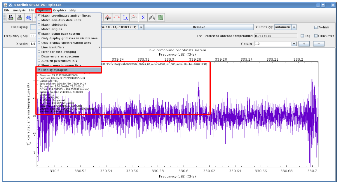
To show or remove the synopsis of a spectrum simply click on the Options button in the spectral view window
and select or deselect Display Synopsis. To move the position of the synopsis simply click and drag the text box
to the desired location.
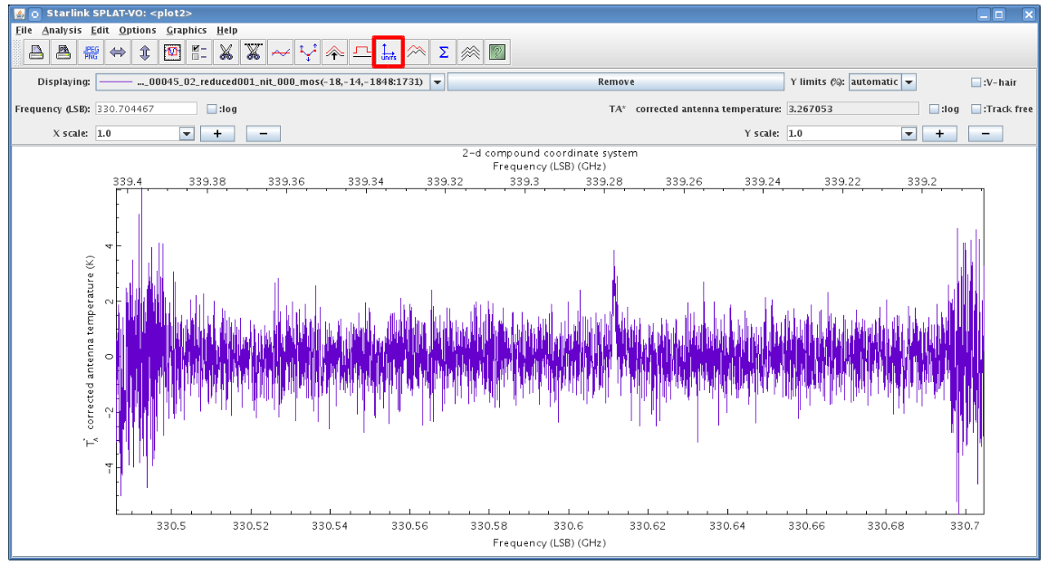
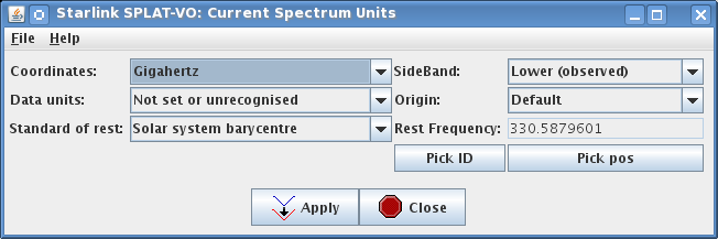
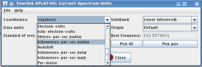
11.3 Changing units of a spectrum in SPLAT
Sometime you may wish to change the units of a spectrum in Splat.
-
(1)
- Click on Change the units of the current spectrum button in your current spectral window.
-
(2)
- A new window will appear called "
Current Spectrum Units".
-
(3)
- From the Coordinates drop-down menu select the desired unit (in this case we select Kilometers-per-sec
(radio)). Then click Apply.
-
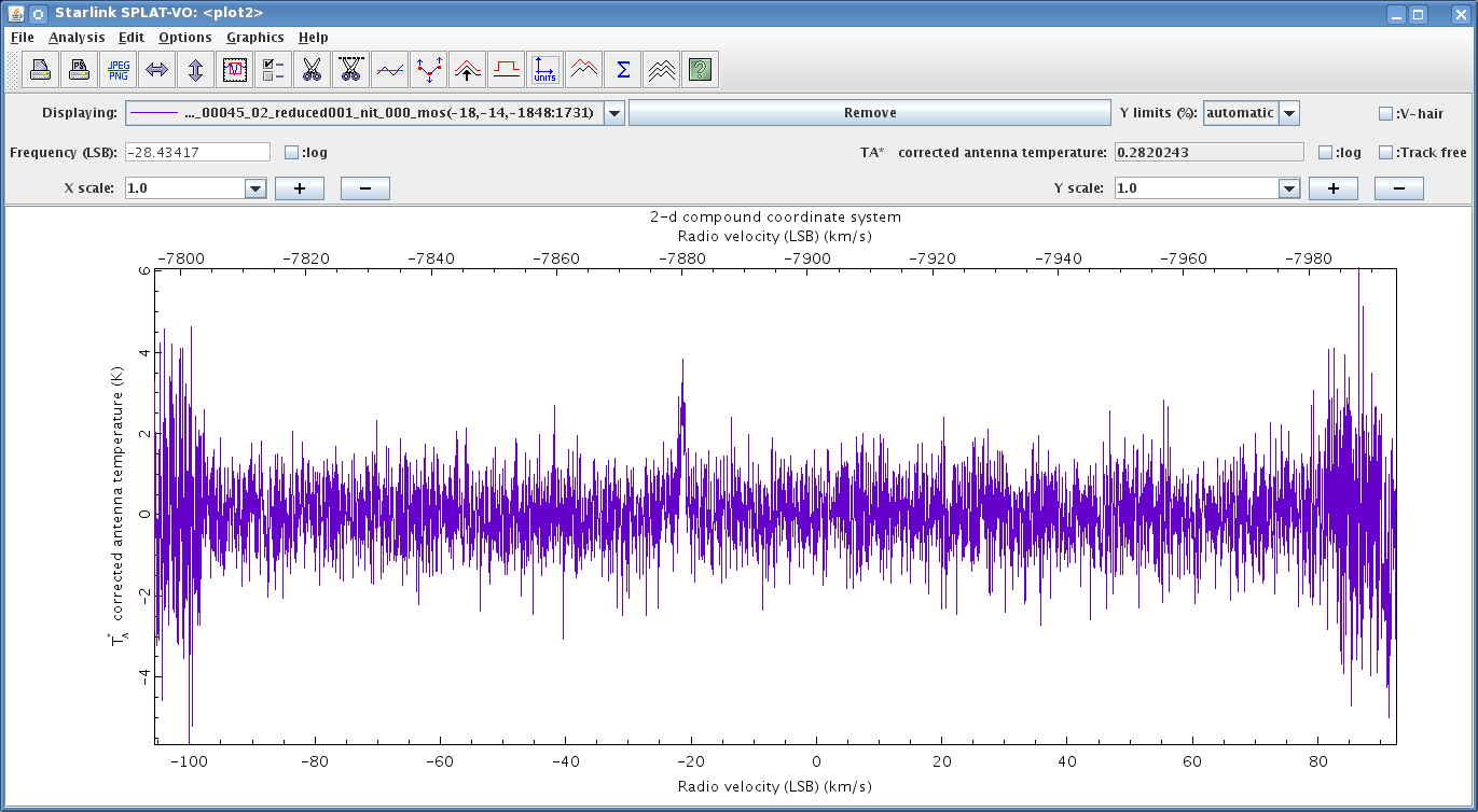
(4)
- You will now see that the spectrum is displayed in Radio Velocity (km/s).
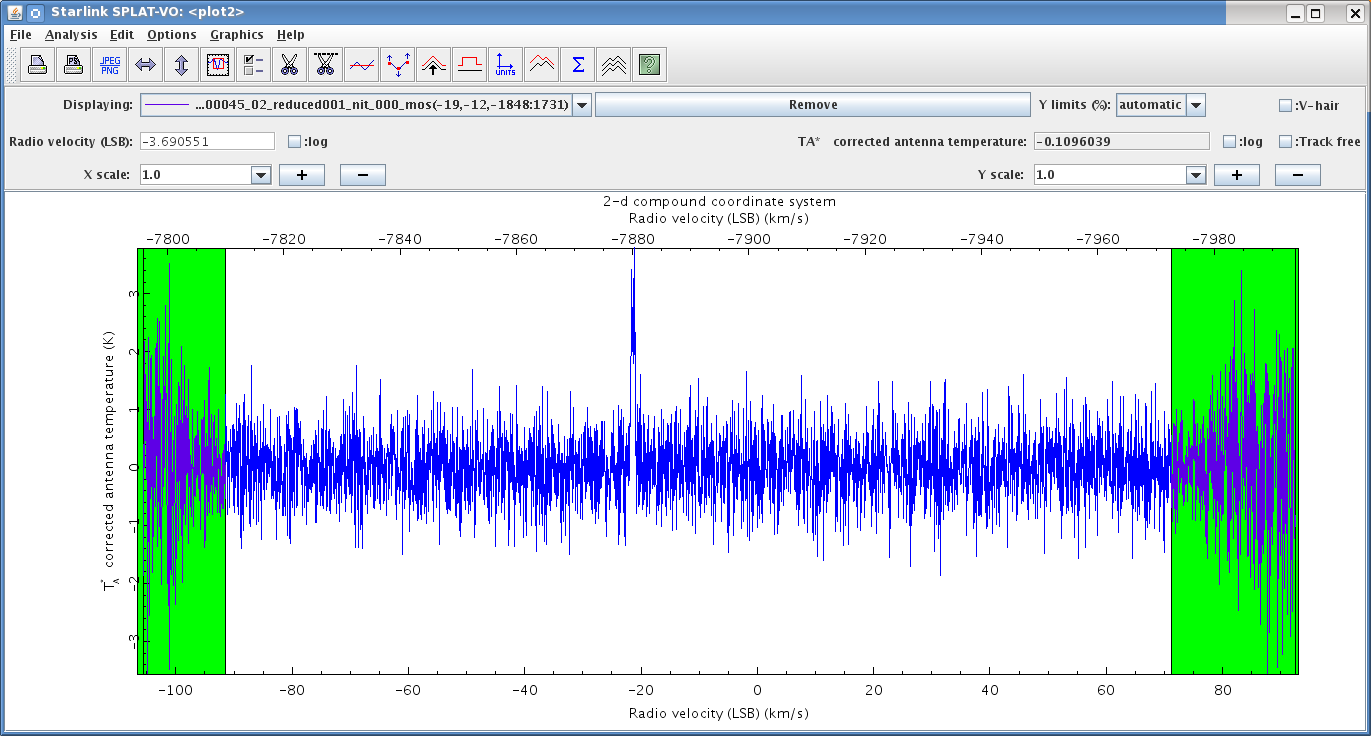
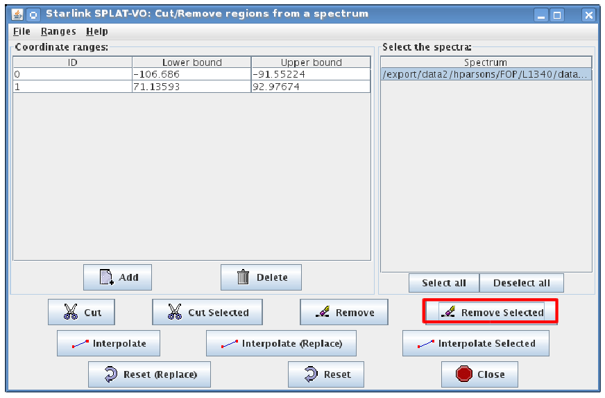
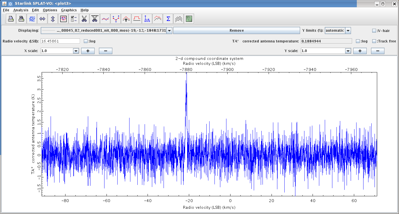
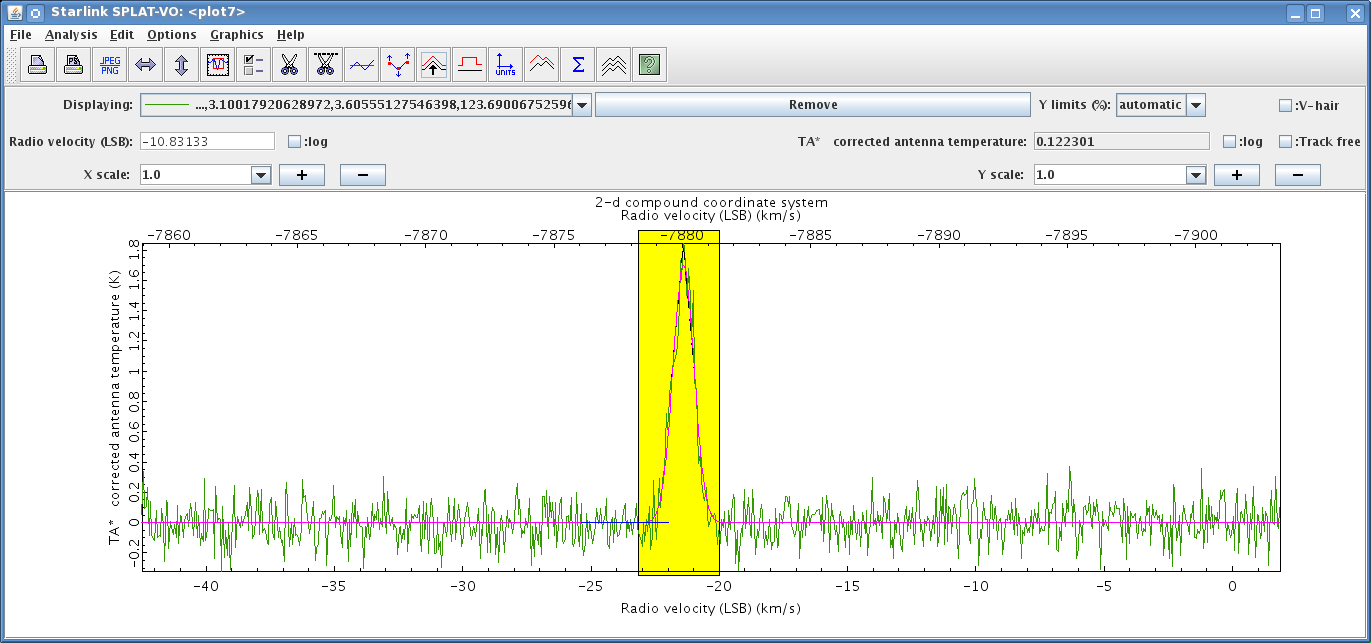
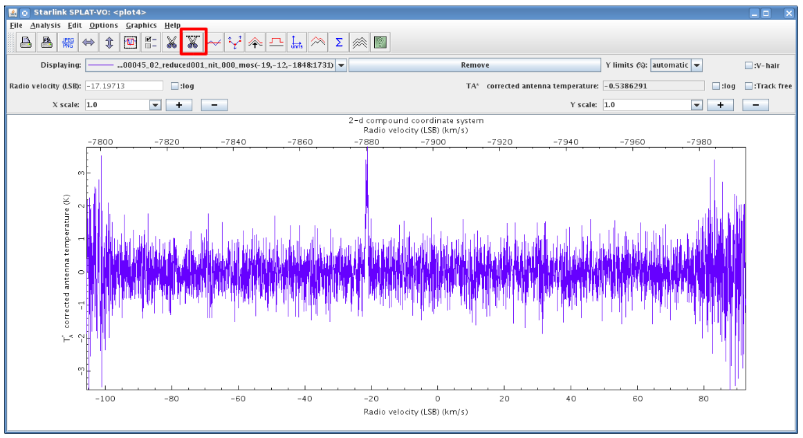
11.4 Cropping a spectrum in SPLAT
-
(1)
- Click on Cut out the regions of the current spectrum button above the spectrum you wish to
work on. This will open a new window.
-
(2)
- Select Add from the cut region window.
-
(3)
- Click and drag the regions you wish to remove from the spectrum in the spectrum window. As we had a
second region to remove we click on the Add button a second time. In this example we select the two noisy
edge regions from the spectrum to remove.
-
(4)
- Select the Remove Selected button.
-
(5)
- A new spectrum with the noisy edges removed will now appear in the main Splat window. Click on your
newly created spectrum to view.
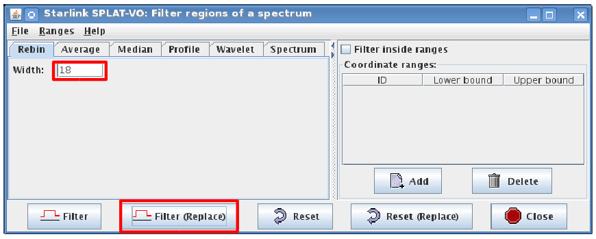
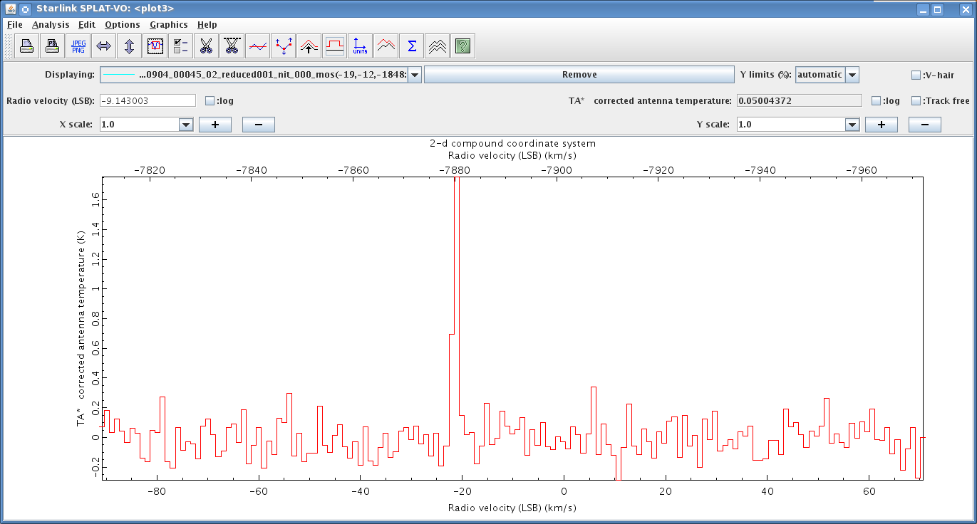
11.5 Rebinning a spectrum in SPLAT
-
(1)
- Click on Apply a filter to the current spectrum button above the spectrum you wish to work on.
This will open a new window.
-
(2)
- Select the number of channels over which you want to bin—this is the Width. In this example the
spectrum has a resolution of 0.055 km s−1.
We bin by 18 channels to rebin the spectrum to 1 km s−1 channels.
-
(3)
- Select Filter (Replace). This will create a new spectrum in the main Splat window and will also
replace the existing spectrum displayed in the spectral window with the new binned spectrum.
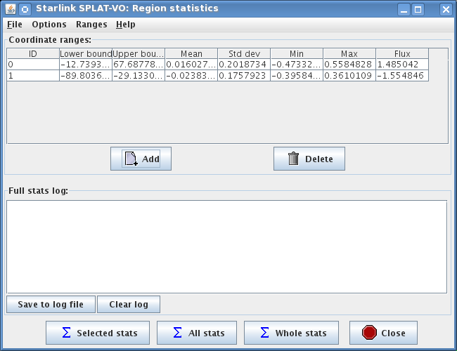
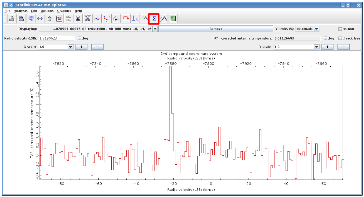
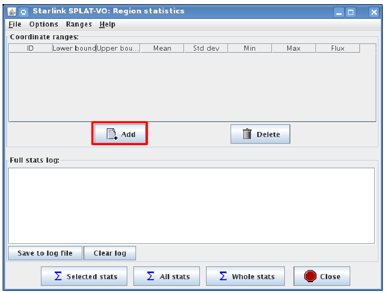
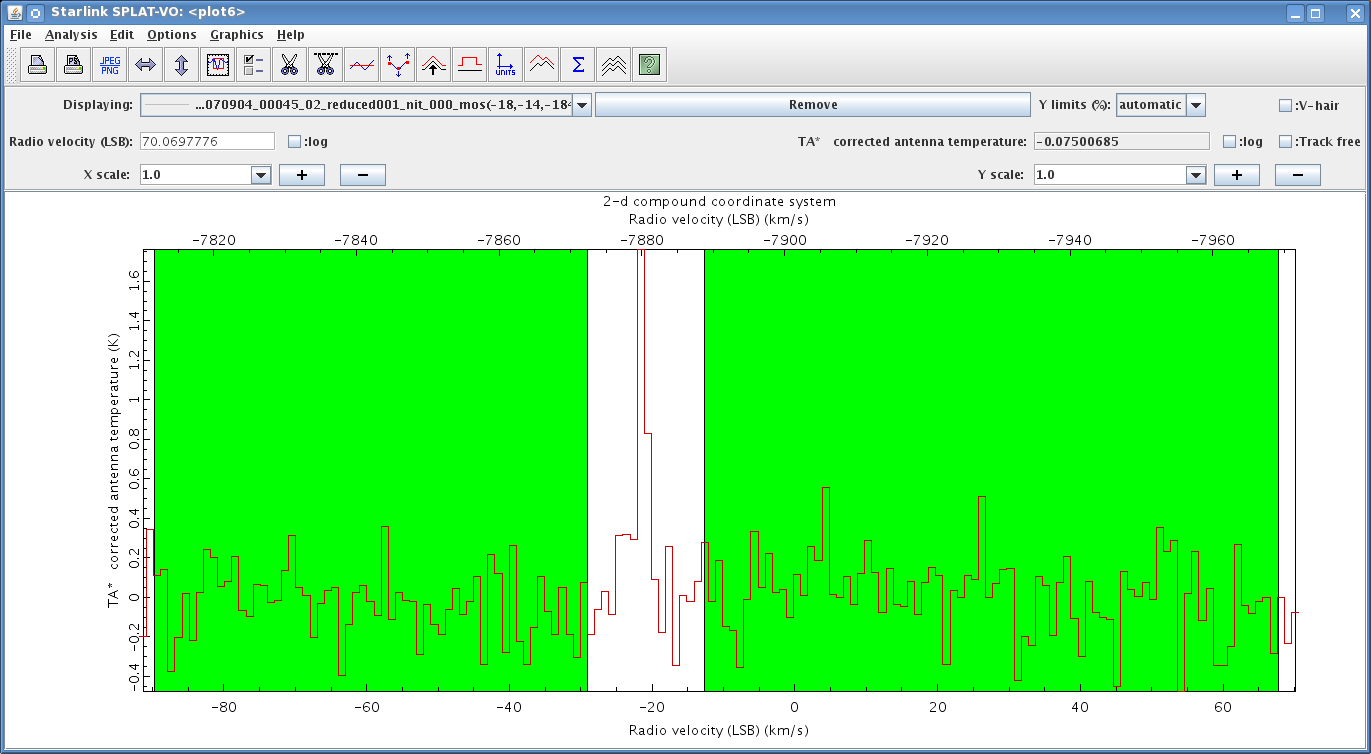
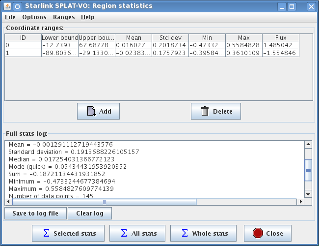
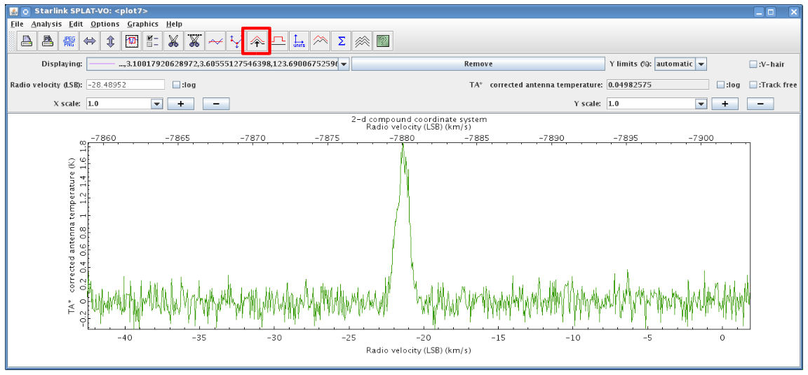
11.6 Estimating the noise in a spectrum using SPLAT
-
(1)
- Click on Get statistics on region of spectrum button above the spectrum you wish to work on.
This will open a new window.
-
(2)
- Select Add from the "
Region statistics" window.
-
(3)
- Click and drag the regions you calculate the statistics over. As we wish to include baselines eithersie of the
spectral line seen in the data we click on the Add button a second time.
-
(4)
- You will see the two selected spectral regions appear in a table in the "
Region statistics" window with
some basic statistic already computed for each region created.
-
(5)
- Click on Selected stats or All stats to get statistics of the regions combined. In this example we see the
standard deviation in the regions selected is 0.19K.
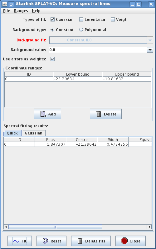
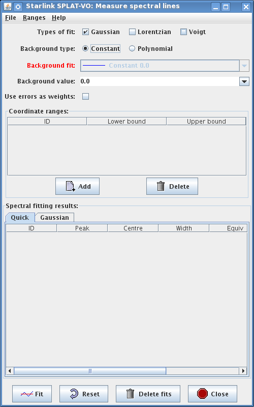
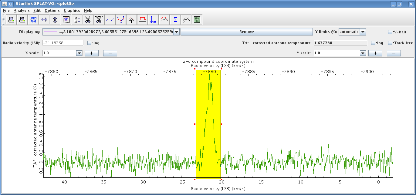
11.7 Fitting a line in a spectrum using SPLAT
Your data might have lines for which you want a quick estimate of its line strength and width.
-
(1)
- Click on Fit spectral lines using a variety of functions button above the spectrum you wish to
work on. This will open a new window.
-
(2)
- Click on the Add button in the "
Measure spectral lines" window.
-
(3)
- Click and drag the box that appears in the spectral window to encompass the line for which you wish to
calculate a fit for.
-
(4)
- Click on the Fit button to produce both a Quick and Gaussian fit to the spectral line.
-
(5)
- We see the results of the fit are provided in the "
Measure spectral lines" window, and the two fits can
be seen in the spectral line window.
Copyright © 2015-2021 Science and Technology Facilities Council,
& East Asian Observatory