Figure 3: A cross-section through a simple spectrum.
In this section each of the basic steps in the spectral data reduction procedure are described. Examples of practical techniques using these ideas are to be found in §5.
Most spectral data will be obtained using a CCD. Careful preparation of CCD data prior to attempting the extraction of science data is essential. In this Cookbook the procedure is outlined (very!) briefly. Those points important to spectral data reduction are included.
The basic steps are:
Depending on your source data and choice of reduction software you may need to:
You may have data which contain dead columns or few-pixel hot-spots. Handling of these is discussed in the documentation for the CCD data preparation packages.
Once a set of arc and object images have been prepared, the data reduction process can begin.
There are several packages for preparing CCD data. All of them offer similar functionality. You’ll find
that it’s easiest to use the package which complements the spectral reduction software you
choose. There are two popular Starlink packages which you might use: ccdpack and figaro.
ccdpack includes some tools for conveniently managing the preparation of many frames
and supports the propagation of errors. It also has a GUI-based interface for setting up
automated reductions. CCDPACK also has better facilities for combination of images, offering
several estimators. In IRAF the noao.imred.ccdred package should be used for CCD data
preparation.
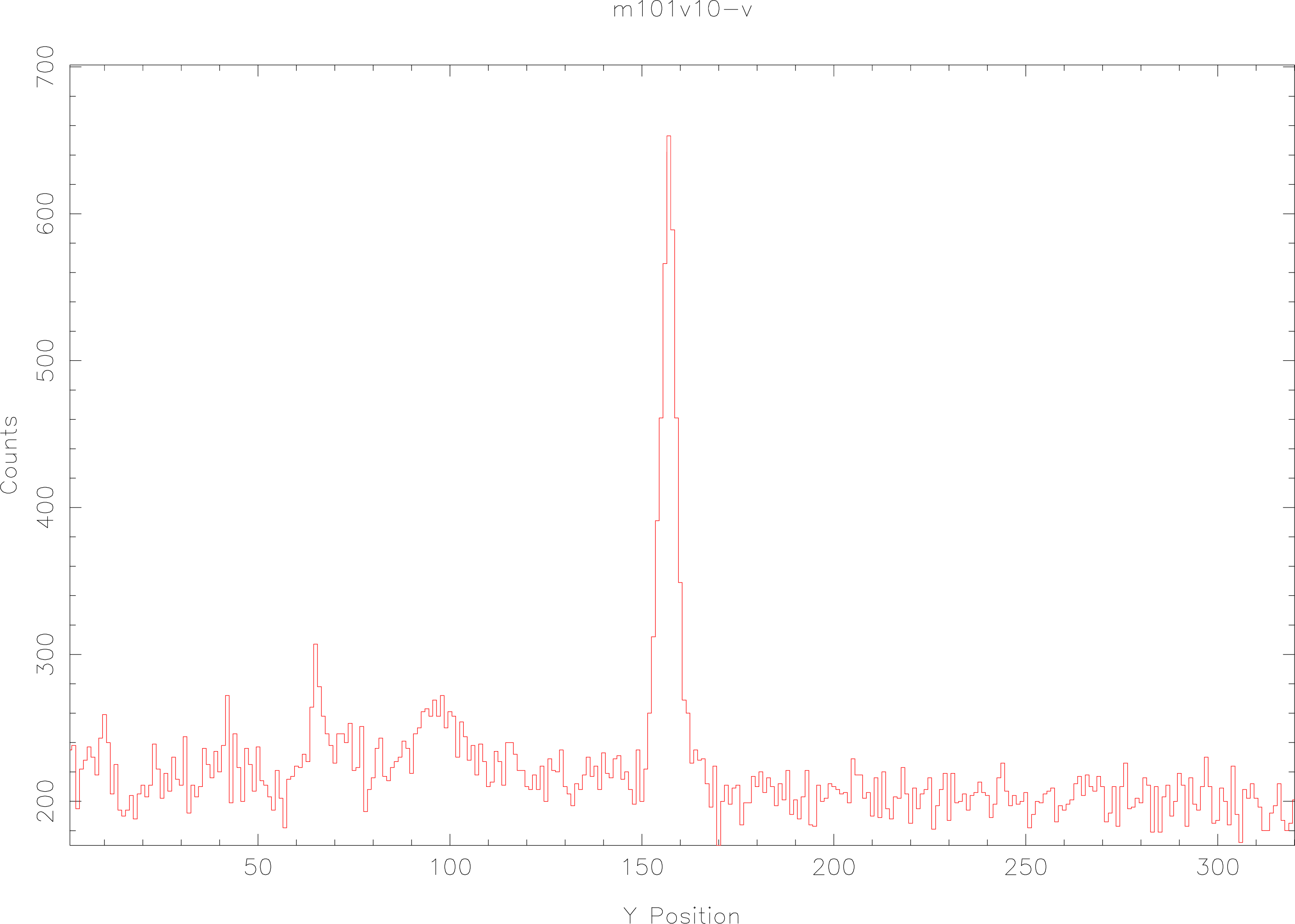
A spectrum running parallel to the X-axis of an image can be located by taking a cross-section (sometimes called a slice or cut) parallel to the Y-axis. For a simple spectrum, a plot of such a section will appear as in Figure 3. If the spectrum is faint, or has strong absorption features, it may be better to take the median of several columns and use this to investigate the spatial profile of the spectrum. This will avoid the case where a single-column section passes through the spectrum and there is no signal as, for example, in a strong absorption feature.
Once we know which row of the image the spectrum is centered on, we can proceed to investigate the spatial profile by re-plotting the cross-section ‘zoomed in’, centred on that row. Figure 4 (left) shows such a plot. The object spectrum has a width at the base of about 18 pixels. We want to sum the signal from 9 pixels to the left of profile centre, to 8 pixels to the right of profile centre to give the gross spectrum for this object. On either side of the spectrum are flatter areas which we have chosen as background channels. We could take the median value of these areas to give a measure of the background. The background level in the object channel can then be estimated by taking the median of these values. In Figure 4, the left-hand background channel runs from 10- to 16-pixels to the left of the profile, and the right-hand channel from 9- to 14-pixels to the right of the profile.
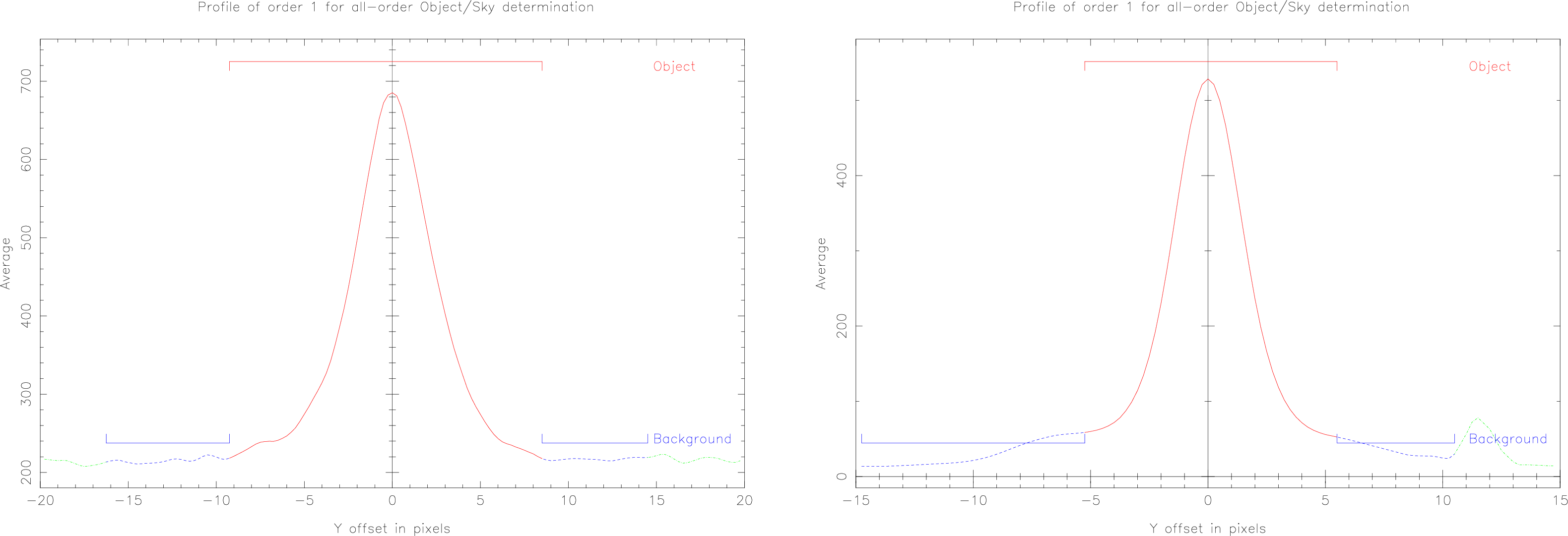
Figure 4 (right) shows a more awkward case, the background is infected, possibly by a cosmic-ray hit, or more likely, by a second, faint object on the slit. In this case the right-hand background channel has been made smaller to avoid the feature. Use as many ‘clean’ background pixels as available—as long as this does not degrade resolution in the dispersion direction (see §4.6). A larger number of pixels gives both a better background estimate, and better rejection of cosmic rays. We might use a linear fit to the backgrounds to allow for the fact that the channels are asymmetrical.
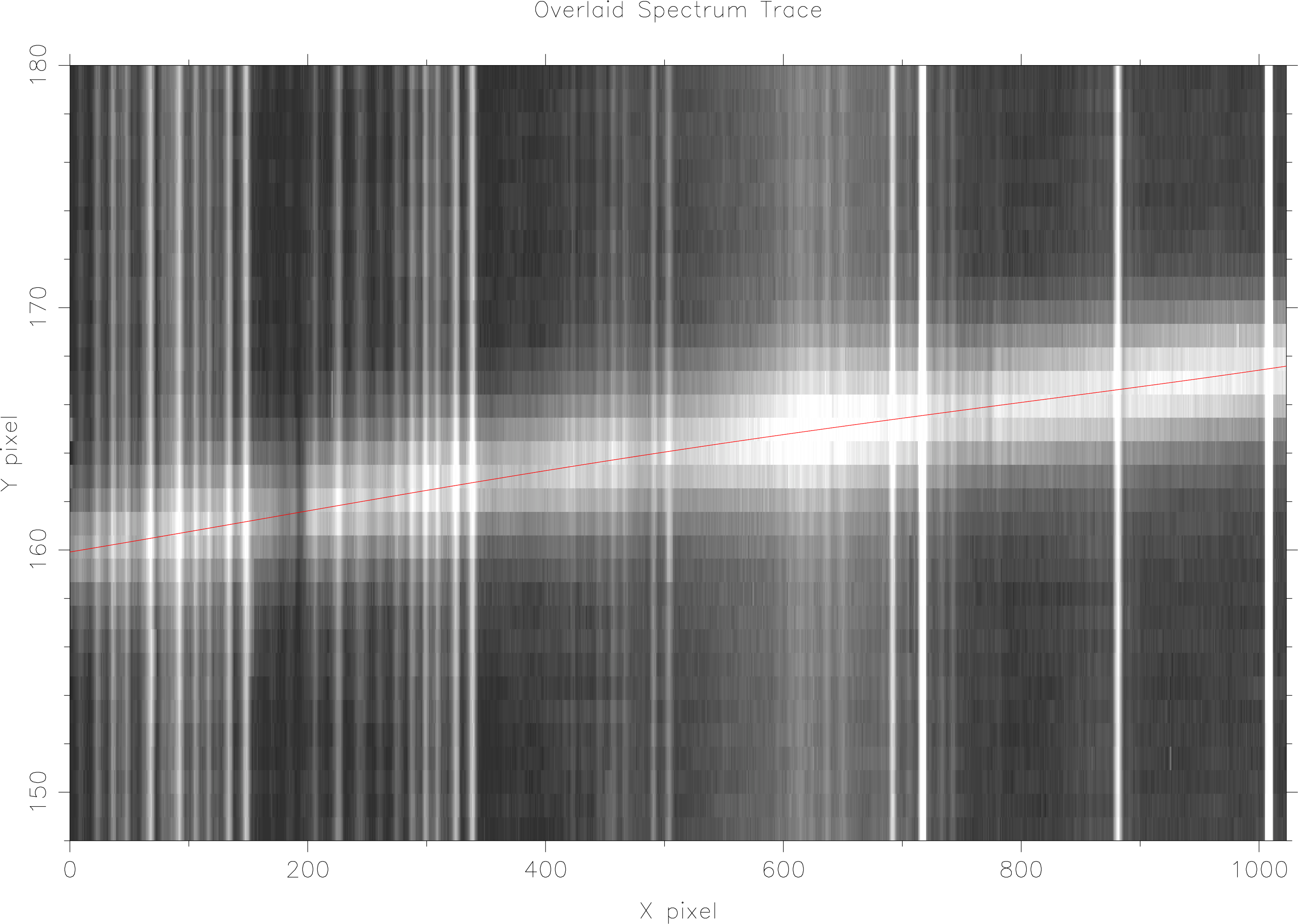
In practice, the spectra produced by an instrument are not aligned precisely parallel to the pixels in the detector used to record them. There are many reasons for this, not least that the effect of atmospheric refraction at the blue and red ends of the spectrum is different. As the position of the centre of the spectrum is subject to shifts in the spatial direction, we need to find the centre of the spatial profile of the spectrum at points along the dispersion direction, and fit a curve to these points. This process is known as tracing the spectrum. Figure 5 shows the curve fitted to a trace overlaid on the image of the spectrum.
When summing the signal from each sample in the dispersion direction, the positions of the object and background channels are re-centered relative to the trace. This ensures that the ‘software slit’ used for the extraction correctly samples the spectrum.
For a bright spectrum with a continuum, tracing is done easily; however, if the spectrum has strong absorption features or is very faint, it can be difficult to find the trace centre along the whole length of the spectrum. There is no perfect way to overcome this problem. The strategy you adopt in these cases will depend upon which frames you have available; it may be adequate to use a flat-field with the dekker stopped down; it may be adequate to use a bright reference star image. As long as you have one frame which you can trace you can use this as a template for the extraction. The template trace may have to be shifted to register with the science frames. You can determine if this is needed by over-plotting the trace on the science frame and inspecting the fit. In the worst case of no frame proving suitable for tracing, the trace path may be defined manually; try to avoid this if at all possible.
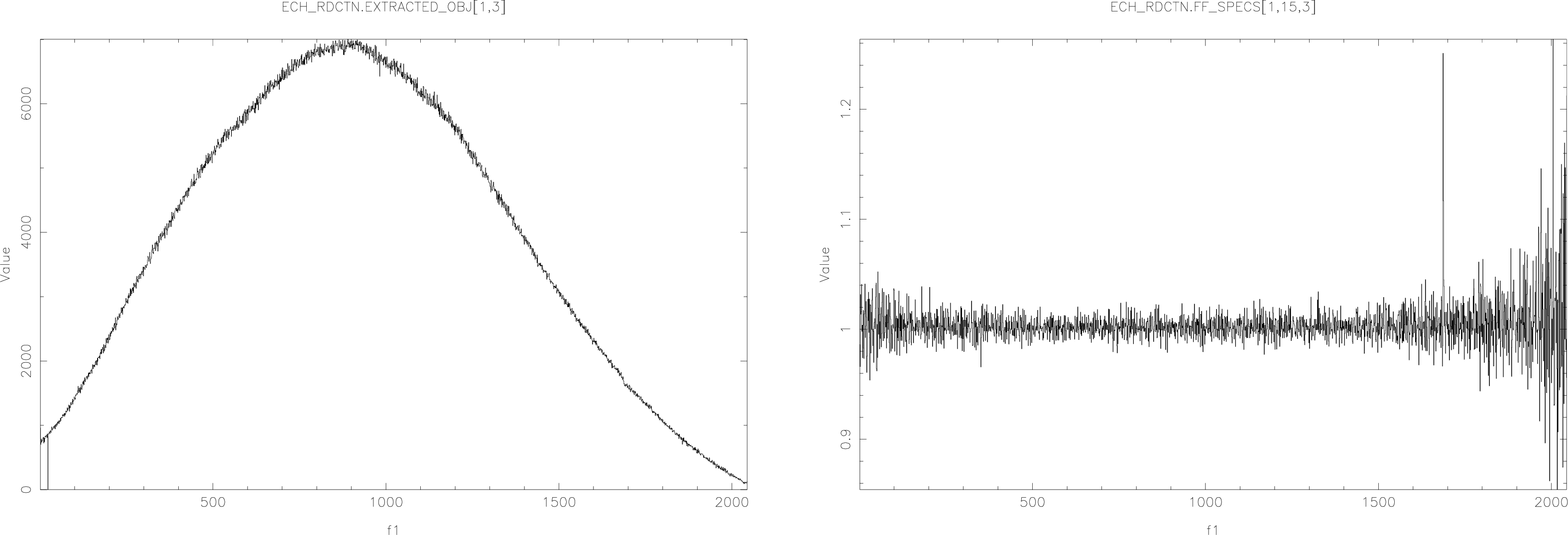
A flat-field frame is needed to correct for the pixel-to-pixel sensitivity variations in the detector (and the small-scale variations in the throughput of the instrument optics). When imaging, an evenly illuminated scene is used as the flat field. For spectroscopy we would want to use a light source which is ‘white’, i.e., the same brightness at all wavelengths. In practice this is not possible and the lamp used for the flat field has some wavelength-dependent variation in brightness. (The effect becomes greater as dispersion increases.) To remove the response of the lamp, a low-order curve is fitted to the response—assuming the spectrum runs with dispersion parallel to the X-axis, we collapse the flat-field frame by summing columns, producing a ‘spectrum’ for the lamp, then fit a curve to this spectrum. Figure 6 shows how one of these ‘spectra’ might appear. The spectrum has a simple, continuous shape with small-scale noise superimposed. Having fitted a curve, we divide the flat-field by it so as to leave the small-scale sensitivity variations only.
In the previous steps nothing has been done to the data; instead, models of the data have been produced. We have:
At this point we are ready to extract the spectrum. The procedure can be very simple, at each sample point along the dispersion direction we sum the signal from all the pixels selected as object; we then subtract a value based upon the pixels in the background channels. The same extraction is applied to both the target and reference star images (if any), as well as to the arc images.
The procedure outlined above is known as a ‘simple’ or ‘linear’ extraction. In many cases such an extraction is adequate; however, this method does not make the most of the data available. A profile curve can be fitted to the spectrum in the spatial direction. At the centre of the profile the signal is greatest; on the outside, the signal falls off to the background level. If we sum these pixels in an unweighted manner we are ignoring the fact that the central pixels have a better signal-to-noise ratio as compared to those at the outside. To overcome this problem we use the so-called ‘optimal’ extraction scheme.
Optimal extraction is suitable for CCD data when we know the readout noise and gain of the CCD camera. The CCD readout noise is needed to calculate pixel weights. The gain is used to convert the data in the input images, which are in the ‘arbitrary’ units from the camera ADC, to units of recorded photons. Once we have the data in these units, we can apply an error-based weighting to the summation of data in each sample along the dispersion direction.
Optimal extraction assumes that a good model for the noise sources in our data is available; this is a fair assumption as the noise sources in a CCD camera system are well understood (well, at least at the sort of level we are interested in anyway). The main noise ‘sources’ are: the camera electronics, the CCD output node, and the shot noise of the electronic charge stored in a pixel (which represents the light signal). There are other sources—see Horne[10] and Marsh[13] for more details of the theory of optimal extraction.
In cases where the CCD parameters are not available, a profile-weighted extraction might be used. This weights the summation of the object pixels based upon their relative brightnesses. This should give a better signal-to-noise ratio than the simple extraction.
Which extraction scheme you select will depend on the nature of—and what you want from—your data. For bright, high signal-to-noise data there is little to be gained by going for an optimal extraction (little may be lost by doing one though…). Optimal-extraction algorithms require that the spatial profile of the object is a smooth function of wavelength. This means that optimal extraction is unlikely to be useful if spatial resolution is required and/or the spatial profile of the object varies rapidly with wavelength, as for objects with spatially-extended emission-line regions. For suitable data, optimal extraction also acts as a cosmic-ray filter: any pixel which deviates strongly from the profile model is likely to be contaminated, and can be rejected.
Once the spectrum extraction is complete we have a two-dimensional dataset: sample number and intensity. (You may also have error data for each sample.) Sample number is simply an index for each integration bin along the spectrum (e.g., the X-axis in Figure 8). For some purposes this spectrum may be enough, but usually the next step in the reduction process is to find the relationship between wavelength and sample number.
The basic steps here are:
You should find that a list of spectral-feature wavelengths for common arc reference lamps is available on-line (see §5.9 for more details). You may also be able to lay your hands on a hardcopy of a ‘mapped’ comparison spectrum for your selected arc lamp, perhaps obtained using the same spectrograph as your data, this will consist of a plot (or series of plots) of the spectrum annotated with rest wavelengths. For example, Bessell & Pettini[4] should be available at most UK Starlink sites. Some people prefer the ESO arc-line atlas[3] in which the line wavelengths are easier to read.
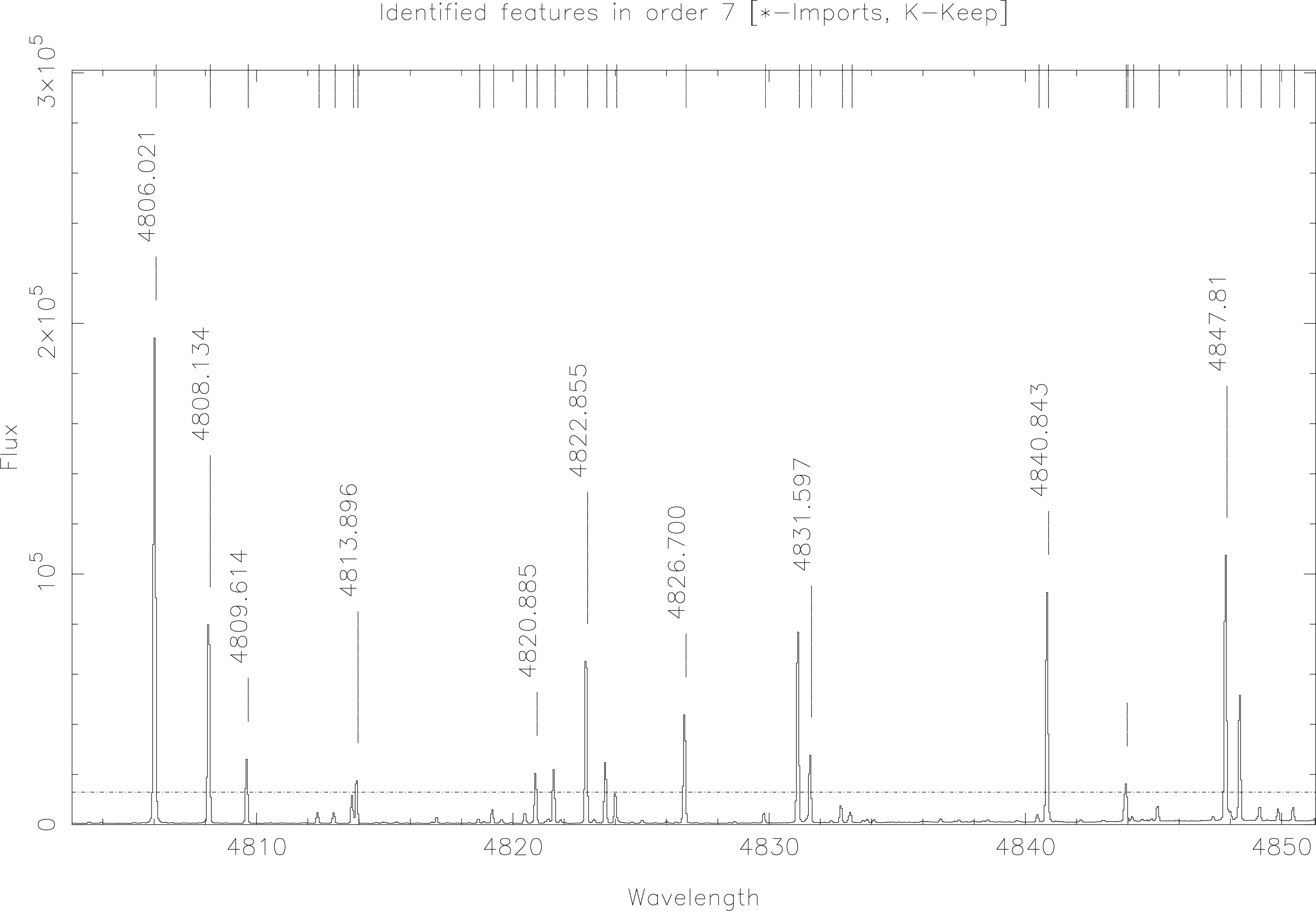
Ideally an arc spectrum should contain at least three or four identifiable spectral lines, preferably with one close to each end of the spectrum, and one or more spread in the middle. In some cases it may be useful to refer to the object and/or reference star spectra to look for strong features of known, or approximately known, wavelength. These can be used to help you ‘home-in’ on features in the arc spectrum. When a fit is made to these features you will be advised of the goodness-of-fit, usually in the form of a plot of line versus deviation-from-fit or RMS deviation values for each line. You will be able to adjust the fit and reject any lines which seem to have been mis-identified, then re-fit the data.
Figure 8 shows a plot of a single order during interactive line-identification using echmenu.
Once you have a complete wavelength-calibrated comparison spectrum you can ‘copy’ the wavelength scale onto your object spectra. It may be useful to calibrate two arcs which bracket the object exposure in time. This will show any time-dependent variation in the wavelength scale. If there is some change (and it is reasonably small) you can take a time-weighted mean of the two bracketing wavelength scales and use this for the object spectrum.
Once you have a wavelength-calibrated spectrum you may (again) be happy enough and not need to go any further. It is more likely that you will want to do one of two things, either flux calibrate, or normalise the spectrum.
If, as part of your observing programme, you take spectra of standard stars then you will be able to attempt to flux calibrate your data.
The flux-calibration process is simple: you compare the extracted standard-star spectrum to a published spectrum of the same star. At each ‘wavelength’ (I use the term very loosely here—see below for a proper explanation) you find the ratio of the observed to published spectrum. The result is a conversion factor at each ‘wavelength’. To flux calibrate your target objects you multiply the spectra by these per-wavelength conversion factors. The effect of this is to remove instrumental-response wavelength-dependency. At least that’s the idea… in practice, you must be careful to understand how the published standards are tabulated, and how this might relate to your data. How Standards are Tabulated There are two ways in which the standard-star data are tabulated, both are tables of fluxes versus wavelengths: in one, each point has a corresponding pass-band width; in the other, each point is a fit to a continuum curve. In the first case, the published standard and your observed standard should look the same once the flux in the appropriate pass bands has been summed—even when absorption features are present in the spectrum. In the second case you must either fit a continuum to your data or, if there are no absorption features present in the wavelength range covered, you might just interpolate between the points in the published standard. Air mass & Extinction The Earth’s atmosphere absorbs and reddens light from astronomical sources. The effect is dependent upon many factors: weather, observing site, time of year, time of day (or night), and so on. The process is known as atmospheric extinction. The depth of atmosphere through which an object is observed is another factor determining the extinction. This depth is known as air mass. When an object lies at the zenith the depth of atmosphere through which it is observed is one air mass. As the zenith angle of the object increases, so does the air mass. The effect of extinction is wavelength-dependent and so a table of correction factors is required. Each observatory should have such a table available for its site. You should observe your standard star through as similar an air mass to the target as possible. Unless the standard is very close to the target, and both are at a fairly high altitude, you may still need to compensate for differential extinction, rather than simply assuming the atmosphere has the same effect on both observations. It may be a good strategy to observe your standards at a range of different altitudes throughout a night, then fit a curve to these and interpolate to calibrate the science observations. If you are fortunate, the air mass for a particular observation will automatically be present in the FITS headers of your data—otherwise you will have to calculate it.
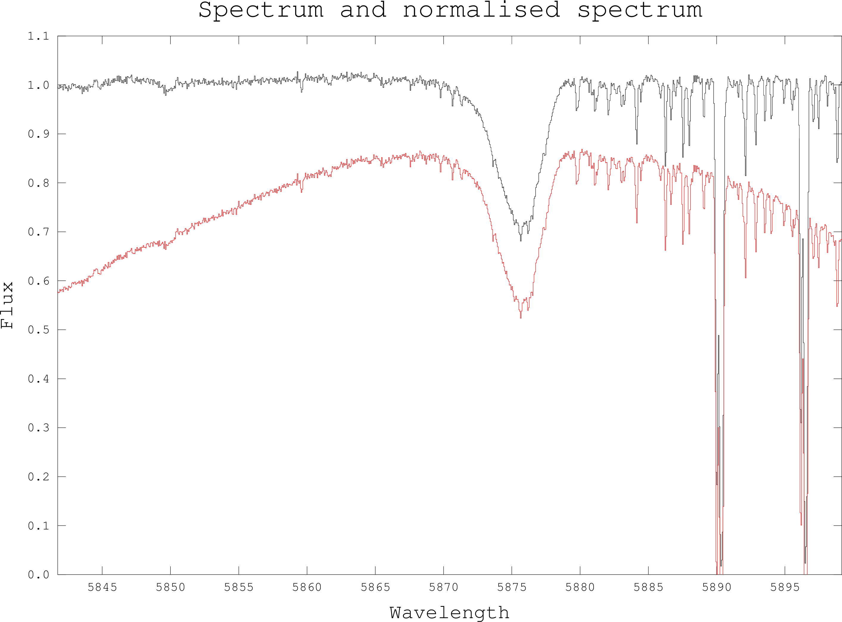
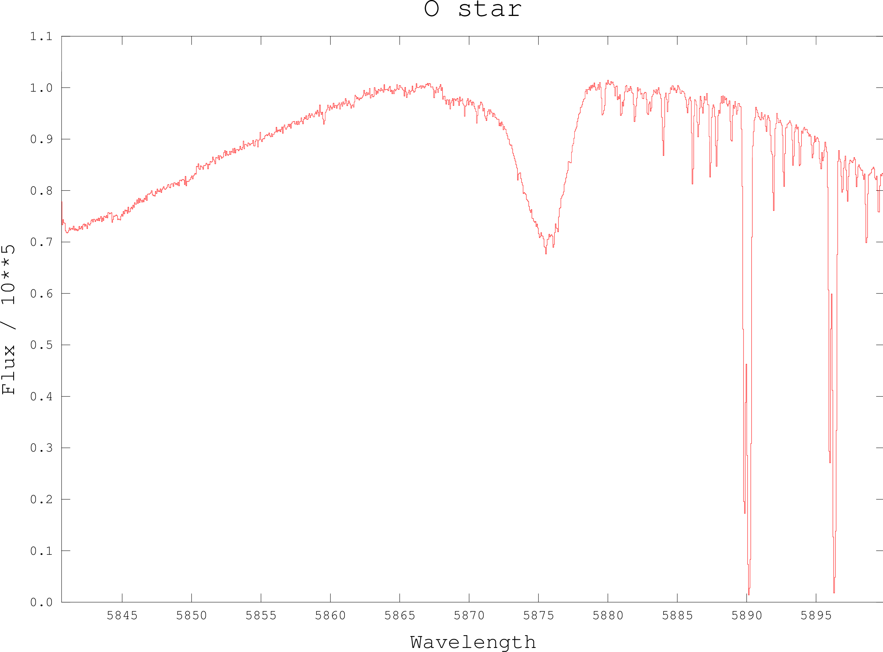
If you are not flux calibrating your data then you will probably want to remove the low-frequency instrument profile from the data. This process is known as normalisation or blaze correction. Figure 9 shows a plot of a spectrum and the same spectrum after normalisation. The continuum is more or less flat in the corrected spectrum. Normalisation can be useful when you want to look at absorption line profiles, model their shapes, or determine their widths.
There are several approaches to normalising the data. One method is to fit a polynomial or other curve to the spectrum and then divide it by the curve. This often works; however, it may well be necessary to manually select which parts of the spectrum to fit as strong spectral features will lead to a poor fit to the continuum. Another method is to ‘draw’ points of the continuum on to a plot of the spectrum and fit a curve to these points. This is usually an entirely manual process.
Another method is to fit a curve to the extracted ‘spectrum’ of a flat field and use that for normalisation. As for the object spectra, this method will only work if the flat-field is devoid of strong spectral features (which it should be, otherwise it isn’t much use for flat-fielding).