Appendix B
SCUBA-2 Data Calibration

B.1 Flux-conversion factors (FCFs)

Primary and secondary calibrator observations have been reduced using the specifically designed dimmconfig_bright_compact.lis. The maps produced from this are then analysed using tailor-made Picard recipes. For instructions on applying the FCFs to your map see Section 8.1 and Appendix E.

A map reduced by the map-maker has units of pW. To calibrate the data into units of janskys (Jy), a set of bright, point-source objects with well-known flux densities are observed regularly to provide a flux conversion factor (FCF). The data (in pW) can be multiplied by this FCF to obtain a calibrated map. The FCF can also be used to assess the relative performance of the instrument from night to night. The noise equivalent flux density (NEFD) is a measure of the instrument sensitivity, and while not discussed here, is also produced by the Picard recipe shown here. For calibration of primary and secondary calibrators, the FCFs and NEFDs have been calculated as follows:

(1)

The Picard recipe SCUBA2_FCFNEFD takes the reduced map, crops it, and runs background removal. Surface-fitting parameters are changeable in the Picard parameter file.

(2)

It then runs the Kappa beamfit task on the specified point source. The beamfit task will estimate the peak (uncalibrated) flux density and the FWHM. The integrated flux density within a given aperture (30-arcsec radius default) is calculated using Photom autophotom. Flux densities for calibrators such as Uranus, Mars, CRL 618, CRL 2688 and HL Tau are already known to Picard. To derive an FCF for other sources of known flux densities, the fluxes can be added to the parameter file with the source name (in upper case, spaces removed): FLUX_450.MYSRC = 0.050 and FLUX_850.MYSRC = 0.005 (where the values are in Jy), for example.

(3)

Three different FCF values are calculated:

(a)

The Arcsecond (Aperture) FCF

$$\mathrm{FC<msub><mrow>F</mrow><mrow>arcsec</mrow></msub>}=\frac{S_{\mathrm{tot}}}{P_{\mathrm{int}}\times A_{\mathrm{pix}}}$$

(B.1)

where $S_{\mathrm{tot}}$ is the total flux density of the calibrator, $P_{\mathrm{int}}$ is the integrated sum of the source in the map (in pW) and $A_{\mathrm{pix}}$ is the pixel area in arcsec${}^2$, producing an FCF in Jy/arcsec${}^2$/pW.

(b)

The Beam (Peak) FCF

$$\mathrm{FC<msub><mrow>F</mrow><mrow>beam</mrow></msub>}=\frac{S_{\mathrm{peak}}}{P_{\mathrm{peak}}}$$

(B.2)

producing an FCF in units of Jy/beam/pW. The measured peak signal here is derived from the Gaussian fit of beamfit. The peak value is susceptible to pointing and focus errors, and we have found this number to be somewhat unreliable, particularly at 450 $\mu$m.

(c)

The Beammatch FCF This FCF is calculated in the same way as the Beam FCF decribed above, but after a matched filter is applied to the data (see Appendix D). This FCF is less commonly used than the former two types.

For a true point source, the measured peak pixel in a map calibrated in units of Jy/beam (using the Beam FCF) is equivalent to the integrated total flux of the same source in a map calibrated in units of Jy/arcsec${}^2$ (using the Arcsecond FCF). The Orac-dr processing routine will automatically select the appropriate FCF based on the default data-reduction recipe that was linked to your data at the time of observations. Note that the data-reduction recipe can easily be changed when running Orac-dr (see Section 4.4.2 for details).

B.2 Extinction correction

Starlink automatically applies the following multiplicative extinction correction to SCUBA-2 data:

where ${\tau }_{\nu }$ is the opacity at the given frequency, $\nu$.

The atmospheric opacity at SCUBA-2’s operating frequencies are defined in terms of the opacity at 225 GHz. Optimizing the uniformity of the SCUBA-2 secondary calibrator fluxes as a function of atmospheric transmission has allowed calculation of the atmospheric opacity relationships for the SCUBA-2 450 $\mu$m and 850 $\mu$m pass-bands to be determined. Full details of the analysis and on-sky calibration methods of SCUBA-2 can be found in Dempsey et al. (2013) [8][9] with updated relations provided in Mairs et al. (2021) [16].

Archibald et al. (2002) [1] describes how the Caltech Submillimeter Observatory (CSO) 225 GHz opacity, ${\tau }_{225}$, relates to SCUBA opacity terms in each band, ${\tau }_{450}$ and ${\tau }_{850}$. The JCMT water-vapour radiometer (WVM) uses the 183 GHz water line to calculate the precipitable water vapour (PWV) along the line-of-sight of the telescope. This PWV is then input into an atmospheric model to calculate the zenith opacity at 225 GHz (${\tau }_{225}$). Historically, this has allowed for ease of comparison with the adjacent CSO 225 GHz tipping radiometer.

The updated opacity relationships (to be used in Equation B.3) derived by Mairs et al. (2021) [16] have been adopted as the default as of Starlink Release 2021A:

and

Previously, (Starlink Versions 2018A and before) adopted as defaults the opacity relationships found by Dempsey et al. (2013) [8]:

and

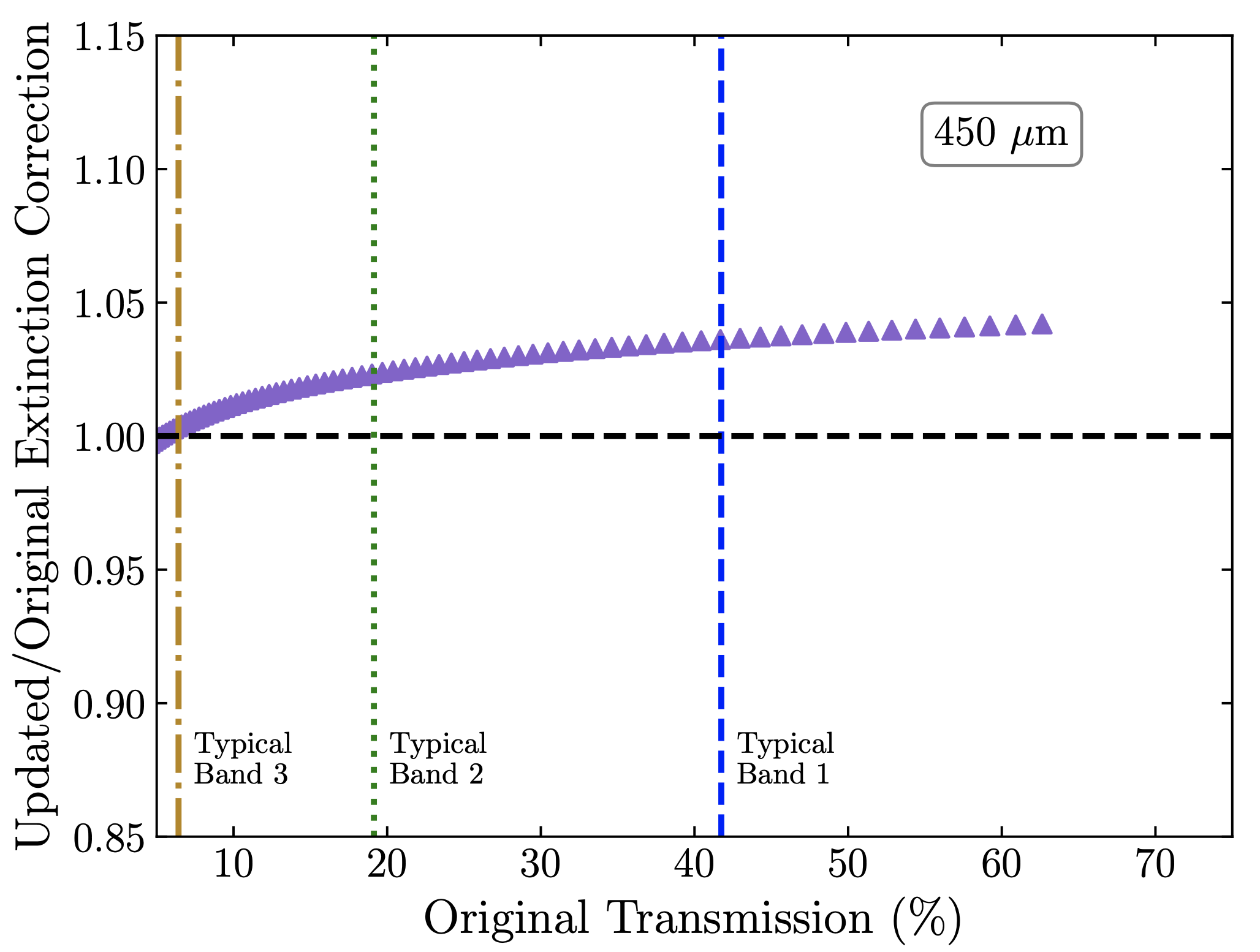
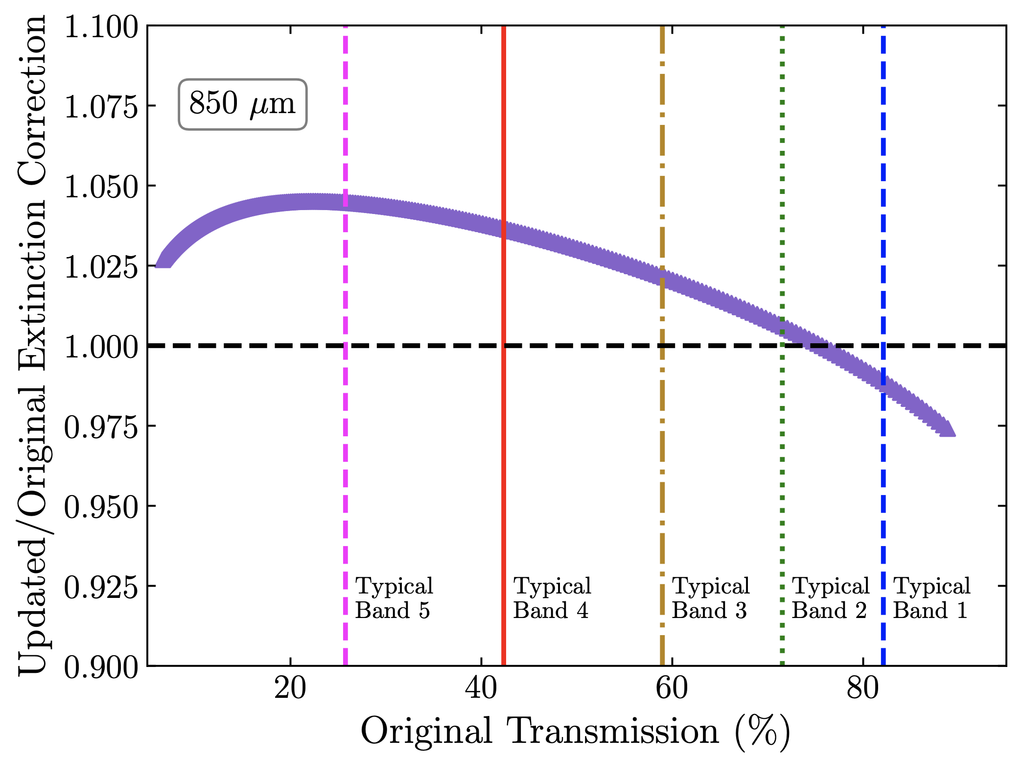
The updated opacity relationships as of Starlink Release 2021A will affect 450-$\mu$m data obtained in very dry conditions and 850-$\mu$m data obtained in very dry or very wet conditions by up to 5% (see Figure B.1).

Note that the default extinction corrections are intrinsically connected to the default FCFs applied. If applying extinction corrections derived by Mairs et al. 2021 ([16]), the matching FCFs must also be applied (see Appendix E). The Orac-dr software assumes the Mairs et al. (2021) [16] results beginning in Starlink Release 2021A. Starlink Release 2018A and previous versions assume the Dempsey et al. 2013 [8] values by default.

Figure B.1: The new extinction corrections derived by Mairs et al. (2021, [16]) divided by the original extinction corrections (Dempsey et al. 2013 [8]) as a function of atmospheric transmission. Vertical lines show the atmospheric transmission of the typical JCMT weather bands at each wavelength, assuming an airmass of 1.2. Left: 450 $\mu$m. Right: 850 $\mu$m. At 450 $\mu$m, the original correction is modified by a maximum of 5% in very dry weather while at 850 $\mu$m the original correction is modified by a maximum of 5% in very dry or very wet conditions. The majority of 850-$\mu$m observations, however, require no modification to the original correction and less than 4% of SCUBA-2 data are obtained in weather band 5.

The SCUBA-2 filter characteristics are described in detail on the JCMT website¹.

The extinction correction parameters that scale from ${\tau }_{225}$ to the relevant filter have been added to the map-maker code. You can override these values by setting ext.taurelation.filtname in your map-maker config files to the three coefficients ‘($a$,$b$,$c$)’ that you want to use (following the form ${\tau }_{\nu }=a\times \left({\tau }_{225}+b+c\sqrt{{\tau }_{225}}\right)$), where filtname is the name of the filter). The defaults are listed in $SMURF_DIR/smurf_extinction.def.