Chapter 8
Post-processing Reduction Steps

8.1 Flux-conversion factors

If you are not using the Orac-dr pipeline to reduce your data (i.e. you are manually employing the map-maker as described in Chapter 5), your data come out of the map-maker in units of picowatts (pW). A flux-conversion factor, or FCF, needs to be applied to scale your data from units of pW to janskys (Jy). For more information on calibrating SCUBA-2 data see Dempsey et al. (2013) [8], Mairs et al. (2021) [16], and Appendix B.

Below are the default FCF values as of Starlink 2021A and they apply to data obtained since 2018 June 30. The Orac-dr pipeline automatically accounts for changes in the FCFs for earlier dates (see the important notes below) but manually running the pipeline requires consulting Appendix E for the appropriate values.

8.1.1 Aperture flux

To measure the flux density of extended sources with aperture photometry you should apply the $\mathrm{FC<msub><mrow>F</mrow><mrow>arcsec</mrow></msub>}$(also known as the arcsecond FCF). You can then sum the emission in an aperture. $\mathrm{FC<msub><mrow>F</mrow><mrow>arcsec</mrow></msub>}$ was determined using a 60-arcsec diameter aperture. If your aperture differs from this you should scale your flux accordingly—the scaling factor can be read off the curve of growth (see Appendix G). This graph gives the ratio of aperture flux to total flux for a range of aperture diameters.

$\mathrm{FC<msub><mrow>F</mrow><mrow>arcsec</mrow></msub>}$ is determined using 1-arcsec pixels. For different pixel sizes you will also need to multiply by the pixel size squared for a total flux calibrated in units of Jy. For more information, see Appendix B.

8.1.2 Peak flux

If you want to read off the peak flux from your map or fit a function to estimate the peak brightness, you should apply the $\mathrm{FC<msub><mrow>F</mrow><mrow>beam</mrow></msub>}$ (also known as the peak FCF). When you open your map in Gaia the value of the brightest pixel will be the peak flux of your source. Applying $\mathrm{FC<msub><mrow>F</mrow><mrow>beam</mrow></msub>}$ will result in a map with units of Jy/beam. For point-like or compact sources smaller than the beam (with a Gaussian profile), this peak value will be the total flux density of your source. For more information, see Appendix B.

8.1.3 Manually Applying the FCF

You can apply an FCF value using the Picard recipe CALIBRATE_SCUBA2_DATA. By default, this will multiply your map by 1000$\times$$\mathrm{FC<msub><mrow>F</mrow><mrow>beam</mrow></msub>}$, where the default $\mathrm{FC<msub><mrow>F</mrow><mrow>beam</mrow></msub>}$value is presented at the beginning of Section 8.1 or in Appendix E, depending on the observation date and Starlink version used. This produces a calibrated map with units of mJy/beam.

You can supply a parameter file if you wish to use a different value for the FCF or use $\mathrm{FC<msub><mrow>F</mrow><mrow>arcsec</mrow></msub>}$. For example, the lines below are written in a parameter file called cal.ini to calibrate the data mapinpW.sdf with $\mathrm{FC<msub><mrow>F</mrow><mrow>arcsec</mrow></msub>}$=2.07:

The default SCUBA-2 FCF will be used if not given and FCF_CALTYPE may either be BEAM (default) or ARCSEC. The recipe will write out the calibrated file with a _cal suffix and will change the units in the map header.

Note that the recipe will also take account of the pixel size when applying $\mathrm{FC<msub><mrow>F</mrow><mrow>arcsec</mrow></msub>}$.

8.1.4 Determining your own flux-conversion factors

Calibration observations are obtained at various points throughout the night and each individual observation can be used to determine FCF values. As noted in Mairs et al. (2021) [16], the spread in FCF values observed over periods of months or years is comparable to the scatter that can be observed over an individual night.

There is no obvious parameter that is the singular dominant cause of the inherent scatter in the observed FCFs. The spread is undoubtedly affected by a combination of:

(1)

The bright and variable atmosphere including subtle effects such as the submillimeter seeing, wind speed, ambient-temperature changes, humidity and low-lying variations in weather conditions with scale heights comparable to several times the height of the JCMT.

(2)

The stability of the WVM calibration.

(3)

Dish instability producing variations in the beam profile.

(4)

Instrumental noise, non-cooled optical components, and uncertainties in the MAKEMAP routine’s modeling and removal of noise components from the time stream.

We therefore recommend caution if you are calculating your own FCF values to apply to data on a given night and suggest using the default values supplied above or in Appendix E, depending on the observation date. Nevertheless, below are instructions on how to perform an investigation into the FCFs calculated from the calibrator observations performed close in time to your obtained science data:

(1)

Reduce the calibrator with the map-maker using dimmconfig_bright_compact.lis as the configuration file.

(2)

Determine the FCF value by passing the output map to the Picard recipe SCUBA2_CHECK_CAL.

  % picard SCUBA2_CHECK_CAL 850calibrator.sdf

This will produce a log file (log.checkcal) which records the both $\mathrm{FC<msub><mrow>F</mrow><mrow>beam</mrow></msub>}$ and $\mathrm{FC<msub><mrow>F</mrow><mrow>arcsec</mrow></msub>}$. Check that these values closely approximate the standard FCF values given above (to a reasonable margin within the uncertainties).

8.2 Cropping your map

The nature of the scan patterns results in SCUBA-2 maps significantly larger than the requested size. The high noise towards the outer edges is a consequence of the scanning pattern. Although this excess data are down-weighted during reduction by the map-maker, you may wish to remove it before either combining maps (see Section 8.3) or publishing your map.

You can crop your map to the map-size set in the data header or to any requested size of box or circle using the Picard recipe CROP_SCUBA2_IMAGES. The centre of the cropping area will always be the centre of your map.

The example above includes a parameter file specifying the radius of the circle to be extracted (in arcsecs). The format for the parameter file is shown below.

If this parameter file is omitted it will default to a box of sides equal to the map size in the header (as requested in the MSB). The output from CROP_SCUBA2_IMAGES is a file with the suffix _crop. Full details of this recipe can be found in the Picard website¹

8.3 Co-adding multiple maps

You may have multiple maps of the same source which you would like to co-add. Picard has a recipe called MOSAIC_JCMT_IMAGES that co-adds maps while correctly dealing with the exposure time and weights NDF extensions. The images are combined using inverse-variance weighting and the output variance is derived from the input variances.

This creates a single output file based on the name of the last file in the list, and with a suffix _mos.

There are a number of options associated with MOSAIC_JCMT_IMAGES (see the Picard manual for a full description). However, the main one is choosing between wcsmosaic (default) and the Ccdpack option makemos for the combination method. For more information on makemos and advice on choosing the best method see SUN/139.

The example parameter file below chooses makemos using a 3-$\sigma$ clipping threshold.

Currently there is no advantage in terms of data quality to reducing all observations simultaneously or separately. However, the latter does allow the option of assessing the individual maps before co-adding.

8.3.1 Registering maps

You can register a series of SCUBA-2 maps to a common reference position using the Picard recipe SCUBA2_REGISTER_IMAGES. This is only possible if a there is a common, known source that is present in all of the input maps. This should be done before combining your maps.

Here the parameter file contains the equatorial position of the reference source as in the example below. See SUN/265 for more details.

REGISTER_X and REGISTER_Y may also be galactic longitude and latitude respectively, both measured in decimal degrees.

8.4 Sensitivity

8.4.1 Getting the noise

You can use the Picard recipe SCUBA2_MAPSTATS to get the noise. This recipe estimates the RMS from both the map, the NEP, and the RMS predicted by the Integration Time Calculator. It then writes out a series of results in a log file called log.mapstats. The parameters written to this file are listed in Appendix C.

This recipe will report the noise in the same input units provided.

Note: SCUBA2_MAPSTATS is only designed to work on reductions of single observations. On co-added observations it could produce misleading results, or even fail completely to work.

If multiple files are run through SCUBA2_MAPSTATS, either in a single call of PICARD or by repeatedly running PICARD in the same terminal on different files, the results will be appended to the existing log.mapstats file. The final columns — project, recipe and filename — are given to ensure it is clear to users which line of the logfile corresponds to which input file. This table can be viewed in an accessible way by using the Topcat software included in Starlink:

After running the command above, click on “Views” Then “Table Data” to display the table.

Steps for getting the noise in your co-added map

After applying any necessary FCF, SCUBA2_MAPSTATS simply executes the following steps to get the map noise.

(1)

Crop the map to remove the noisy edges.

  % picard CROP_SCUBA2_IMAGES map_cal.sdf

(2)

Run the Kappa command stats to extract the median value from the error array (the ndf extension that describes the uncertainty in each pixel, calculated from the square root of the variances in the raw bolometer data that contributed to the pixel).

  % stats map_cal_crop comp=err order

8.4.2 Map statistics

The Kappa commands histat and stats are very similar and both return a range of statistics describing any NDF. In addition to the main data array they can be passed the error (comp=err), variance (comp=var) or quality (comp=qua) arrays (if available).

The reported statistics include the pixel maximum and minimum, standard deviation, number of pixels used and omitted, along with pixel mode, and mean. If you supply the order keyword, the median is also shown.

Note: the standard deviation of the data array will give a similar result to the mean/median of the error array except with additional contamination from sources.

8.4.3 Viewing the noise histogram

You can view a histogram of the error array with the Kappa command histogram. Again comp=err must be specified.

The output is shown in the Figure 8.1. For more information on the options for histogram see SUN/95.

Figure 8.1: The error array viewed with Kappa command histogram.

8.4.4 Examining the error map with GAIA

It is also useful to view the error map itself. Open your reduced map in Gaia, then select the Error button on the Select NDF in container file window—see Figure 8.2. You will need to adjust the scaling to view the error map properly.

To assess the noise using Gaia, go to the toolbar on the main window and click on Image-Analysis$\Rightarrow$Image regions. Next select the region shape you would like to check and draw it on your map by clicking and dragging the mouse. Click the Stats selected button in the Image regions window to get a report of the statistics in the selected region.

Figure 8.2: The error array displayed with Gaia. After clicking the Error button (circled in red) you will have to rescale your map.

8.5 Regridding your data

To change the pixel size use the Kappa command compave. The following example increases the pixel size from 4 arcsec to 8 arcsec by using a compression factor of 2.

8.6 Displaying masks

SCUBA-2 maps created using “AST-masking” (see Section 3.5) will contain a Quality array indicating the background pixels that were masked (i.e. forced to zero). In itself this is fairly simple—background pixels have a non-zero Quality value and source pixels have a Quality value of zero. However, it is also possible to have independent masks for the FLT and COM models, in addition to the AST mask. For instance, maps created using dimmconfig_bright_extended or dimmconfig_jsa_generic will have Quality arrays that contain both a FLT and an AST mask, and so some care needs to be used when interpreting the Quality array.

Each value in the Quality array is restricted to taking integer values between 0 and 255, and so can be thought of as 8 separate bits. Each “bit plane” within the Quality array holds a single mask—AST, FLT or COM. The showqual command can be used to find out which mask is held by which bit plane:

This means that the AST mask is stored in bit 1 (the least significant bit), the FLT mask is stored in bit 2, and there is no COM mask. Note, if a map was produced using FLT masking but no AST masking, then the FLT mask would be stored in bit 1.

The decimal integer value of any element of the Quality array is equal to the binary value formed from the bits listed by showqual. So in the above case the maximum Quality value is 3 (the decimal equivalent of binary “11”-e–both bits set). Remembering that a bit is set (i.e. is 1) for background pixels and cleared (i.e. is 0) for source pixels, it follows that the four possible decimal Quality values in the above case (0-3) are:

(1)

- neither bit set, so the pixel is inside both the AST and the FLT mask (a source pixel).

(2)

– Bit 1 set, but not Bit 2, so the pixel is outside the AST mask but inside the FLT mask (a border-line pixel).

(3)

– Bit 2 set, but not Bit 1, so the pixel is inside the AST mask but outside the FLT mask (a border-line pixel).

(4)

– Both bits set, so the pixel is inside neither mask (a background pixel).

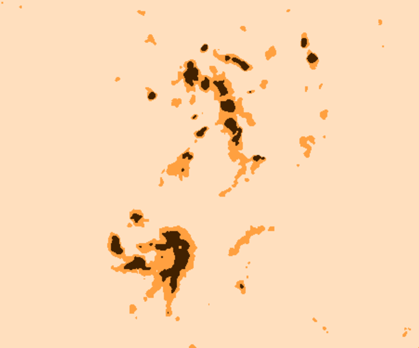
Figure 8.3 shows a simple map of the Quality array values—the black areas have value zero and are thus inside both masks, the dark brown areas have value 2 and are thus inside the AST mask but outside the FLT mask. The light-brown areas have value 3 and are inside neither mask. In this particular case, there are no areas with a quality value of 1, so the FLT mask is contained entirely within the AST mask.

Figure 8.3: The quality component from a typical map.

To produce a plot like this, first open your map in Gaia. Select the top level NDF from list in the pop-up window then click the Quality button. You will need to rescale the map to bring out the masks–see Figure 8.4 for another example showing the full Gaia window (using rather brighter colours this time!).

Figure 8.4: Using Gaia to display the mask applied by the map-maker. Select the QUALITY component of your map.

There are several commands within Kappa that manipulate Quality arrays in various ways. For instance, the setbb command allows pixel data values to be set bad if the associated Quality value has a specified collection of set bits. Thus:

will set all pixels bad in fred.sdf except for those inside the AST mask. Likewise,

will set all pixels bad except for those inside the FLT mask. Note, the change made by setbb is temporary—it can be undone by doing:

To display the fred.sdf map and then overlay the AST mask in blue and the FLT mask in red, do:

The resulting plot is shown in Figure 8.5.

Figure 8.5: The AST and FLT masks contoured together over an image.

Alternatively, Gaia can be used to contour the Quality array over an image, but you cannot then distinguish the AST mask from the FLT mask. First you will need to copy out the QUALITY component of the data to a separate file using ndfcopy:

Then open your map in Gaia and contour the mask NDF on top. Select Contouring... from the Image-Analysis menu, and supply the name of the mask NDF either by entering its name in the Other image: box, or selecting with Choose file... file browser. See Figure 8.6.

For more information on the use of masks by makemap and the parameters that affect them see section 3.5.

Figure 8.6: Using Gaia to display your map with the AST mask used by the map-maker contoured on top.

8.7 Point-source extraction: the matched filter

This effectively fits a single Gaussian point spread function (PSF), centered over every pixel in the map, and applies a background suppression filter to remove any residual large-scale noise.

Cosmology maps usually contain very faint sources that often need extra help extracting. The Picard recipe SCUBA2_MATCHED_FILTER can be used to improve point-source detectability.

The matched filter works by smoothing the map and PSF with a broad Gaussian, and then subtracting from the originals. The images are then convolved with the modified PSF. The output map should be used primarily for source detection only. Although the output is normalised to preserve peak flux density, the accuracy of this depends on how closely the real PSF matches the telescope beam size. In the case of nearby sources, each ends up contributing flux to both peaks.

As in the example parameter file below we have requested the background should be estimated by first smoothing the map and PSF with a 15-arcsec Gaussian.

This is a fairly common technique used throughout the extra-galactic sub-millimetre community to identify potential sources. A full description of the matched filter principle is given in Appendix D, while the Picard manual gives full details of all the available parameters.

8.8 Clump finding

The Cupid application findclumps can be used to generate a clump catalogue. It identifies clumps of emission in one-, two- or three-dimensional NDFs. You can select from the clump-finding algorithms “FellWalker”[2], “Gaussclumps”, “ClumpFind” or “Reinhold” and must supply a configuration file specific to each method. See the Cupid manual for descriptions of the various algorithms.

The result is returned as a catalogue in a text file and as a NDF pixel mask showing the clump boundaries.

The shape option allows findclumps to create an STC-S description (polygonal or elliptical) for each clump that can be displayed over any image in Gaia(Figure 8.7). These are added as extra columns to the output catalogue.

Figure 8.7: STC shapes displayed over the input map with Gaia. To overlay your clumps in this way display your map with Gaia. Under the Image-Analysis menu select Positions... followed by Import CUPID catalogue... In the pop-up window select the .FIT file generated by findclumps and ensure the STC shape box is checked before importing.

8.9 Map provenance & configuration parameters

You may want to check a reduced file to determine which raw files went into it and what configuration parameters were used with the map-maker. There are a number of useful Kappa commands to help you with this:

Map provenance

provshow will list all the NDFs and operations that were used in the creation of your map, while hislist will show a truncated list of input files and operations but will list every configuration parameter used by the map-maker. This includes all the hidden default values as well as those specified in your supplied configuration file. These commands are executed like this:

  % provshow 850map
  % hislist 850map

The output of provshow can be very long. If you merely want to know what the original files were, the ones with no parents, select the root ancestors.

  % provshow 850map show=roots

Map-maker parameters

The task configmeld will compare two maps and highlight any differences between the configuration parameters that were used to create the maps. A configuration file can be supplied in place of a map, in which case the parameters used to create the map are compared with those in the configuration file. configmeld requires a visual-differences tool to be installed on your machine; those currently recognised are: meld opendiff, diffmerge, kdiff3, tkdiff, and diffuse, and are searched for in that order. The follow example illustrates two ways to run configmeld:

  % configmeld 850map1.sdf 850map2.sdf
  % configmeld 850map1.sdf ^mydimmconfig2.lis

Another useful command is the Kappa command configecho. This is very versatile and will display the name and value of one or all configuration parameters either from a configuration file or from the history of an NDF.

The first example below will return the value of numiter from the map 850map.sdf. The second example will display the values of all the parameters in 850map.sdf and will prefix them with a ‘+’ if they differ from the the default parameter values defined in $SMURF_DIR/smurf_makemap.def.

  % configecho name=numiter config=! ndf=850map.sdf
  % configecho name=! config=^$SMURF_DIR/smurf_makemap.def ndf=850map.sdf