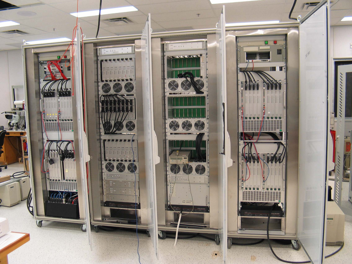
Figure 3.1: Front view of ACSIS at the JCMT. Although designed to work with HARP, ACSIS can be
used with any JCMT heterodyne receiver.
Submillimetre instruments use heterodyne techniques to observe spectral lines at high resolution. Heterodyne receivers take a weak incoming signal and mix it with a reference frequency known as the local oscillator (LO). This results in a signal of lower (intermediate) frequency (IF) which can be amplified and more easily sampled. The current JCMT receivers have a standard IF of 6 GHz for the Nāmakanui insert ‘Ū‘ū, 5 GHz (HARP) and 4 GHz (for the retired RxA) - although these can be adjusted as needed by the user.This mixing produces two frequencies for each value of the LO (νsky=νLO±νIF) which are known as the upper sideband (USB) and lower sideband (LSB).
In a single-sideband receiver (denoted SSB) one of these is suppressed. Double-sideband receivers (denoted DSB) have the two frequencies superimposed. In Sideband Separating mixers (denoted 2SB) both the USB and LSB are generated separately.
Reducing the noise in the system is crucial to the efficiency of these receivers. The required integration time is directly proportional to the total noise in the system given by Tsys via the radiometer formula
where the terms are as follows:
The heterodyne instruments described below are those currently operational, soon to be operational or recently retired at the JCMT. For information on previous instruments see the JCMT web pages.
In the following ηMB is the main-beam efficiency and η fss is the forward spillover and scattering efficiency. For the latest and historical calibrations visit ACSIS Beam Efficiencies.
The Nāmakanui instrument is a spare receiver for the Greenland Telescope (GLT) on loan for use on the JCMT courtesy of ASIAA. Nāmakanui contains three inserts: ‘Ala‘ihi, ‘Ū‘ū, and ‘Āweoweo operating around 86, 230, and 345 GHz. Each of the three inserts receive dual linear polarizations which are labelled using a zero-based system: P0, P1. Each insert has a separate optical path and so only one receiver/frequency range can be used at any one time.
‘Ū‘ū is one of three inserts held within the Nāmakanui instrument. ‘Ū‘ū is a dual linear polarizations Sideband Separating (2SB) instrument. It operates between 215 and 270.6 GHz. It achieved first light on 2019 October 5. The most-common observing mode for ‘Ū‘ū is stare mode, but ‘Ū‘ū is also able to take jiggle and raster maps.
| Receiver | FWHM | ηMB | η fss |
| ‘Ū‘ū | 20″ | 0.57 | * |
‘Āweoweo is another of three inserts held within the Nāmakanui instrument. ‘Āweoweo, like ‘Ū‘ū, is also a dual linear polarizations Sideband Separating (2SB) instrument. It operates across a frequency range that spans between 276 and 371 GHz. ‘Āweoweo saw first light on 2021 January 14. Due to its sensitivity ‘Āweoweo’s most-common observing mode is stare. For larger areas, HARP becomes more efficient for jiggle and raster mapping.
‘Ala‘ihi is the other insert held within the Nāmakanui instrument. Unlike ‘Ū‘ū and ‘Āweoweo, ‘Ala‘ihi is a Single SideBand (SSB) instrument. It will operate at frequencies around 77 to 88 GHz with dual linear polarizations. Its primary function at the JCMT will be as part of VLBI observations.
The Heterodyne Receiver Array Programme (HARP) is single-sideband receiver (SSB) comprised of a 16-receptor array arranged on a 4×4 grid [3]. It operates in the B-band between 325 and 375 GHz. The receptors are adjacent on the focal plane but separated on the sky by 30 arcseconds (or approximately twice the beamwidth). The footprint of the full array is 2 arcminutes. Note that not all receptors are operational; historically between 12 and 15 receptors have been available at any given time. The tracking receptor is chosen to be the best performing of the four internal (2×2) receptors in the grid.
You can find the number of the tracking receptor and the number of working receptors in the FITS header
values REFRECEP and N_MIX respectively.
In addition to stare observations with the tracking receptor, the most common observing modes for HARP are jiggles and raster maps. These observing modes are described in Section 3.3 and an example image from each mode is shown in Figure 3.2.
| Receiver | FWHM | ηMB | η fss |
| HARP | 14′′ | 0.63 | 0.88 |
Receiver A3 (RxA3) was a single-element double-sideband (DSB) receiver. It operates in the A-band between 211 and 276 GHz. In addition to stare observations, the most common observing mode for RxA3 was raster mapping. In 2016 RxA3 was updated to RxA3M. The instrument was retired in 2018.
| Receiver | FWHM | ηMB | η fss |
| RxA3 | 19.″7 | 0.57 | 0.80 |
RxA3M had an additional calibration step (automatically applied by our pipelines if you use a version after June 2019) to normalise the flux levels of observations between the upper and lower sideband. If you need more control of this in the pipeline, please see the calibration recipe parameters in Appendix G. The older RxA3 also had some variation in flux levels between the sidebands, but we do not have a calibration correction for this.
Since 2006 September, the backend for heterodyne instruments has been the Auto-Correlation Spectrometer and Imaging System known simply as ACSIS (see Figure 3.1). Given the various combinations of ACSIS’s 32 down-converter modules and available IF outputs from the different instruments, a number of bandwidth modes and corresponding frequency resolutions are available. Listed below are the most common ones. Visit the JCMT ACSIS webpage for a full list.
| Subbands | Bandwidth mode | Channel Spacing |
| 1 | 250 MHz | 0.0305 MHz (HARP/RxA/RxW) |
| 1 | 1000 MHz | 0.488 MHz (HARP/RxA/RxW) |
| 1 | 1860 MHz (1600,1800) | 0.977 MHz (HARP) |
| 0.488 MHz (RxA/RxW) | ||
| 1 | 440 MHz (400,420) | 0.061 MHz (HARP) |
| 0.0305 MHz (RxA/RxW) | ||
| 2 | any 250 MHz | 0.061 MHz (HARP) |
| 0.0305 MHz (RxA/RxW) | ||
| 2 | any 1000 MHz | 0.977 MHz (HARP) |
| 0.488 MHz (RxA/RxW) | ||
There are a number of special configurations available with ACSIS. These make use of multiple sub-bands to
cover lines at different frequencies. You can find the subsystem number for a given observation by the FITS
header SUBSYSNR.
You will find each subsystem number corresponds to a different molecule or
transition (given by the FITS headers MOLECULE and TRANSITI). For example,
C18O (3-2)/13CO (3-2)
and DCN (5-4)/HCN (4-3) for HARP,
12CO/13CO/C18O
for ‘Ū‘ū,
and with the now retired RxA the common pairing was
SiO (60-50)/SO (43-34).
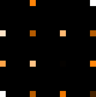


| Stare | A stare, or sample, observation is as simple as it sounds. When you open reduced cubes of stare observations in Gaia you will see a map consisting of one pixel for each receptor; one in the case of ‘Ū‘ū, ‘Āweoweo and RxA, and up to 16 with HARP. The left-hand panel of Figure 3.2 shows a stare observation (taken by HARP) opened in Gaia. You can also view the central spectrum using linplot (see Appendix F) or Splat. |
|---|---|
| Jiggle | A jiggle map is a common HARP observing mode. They are designed to fill in the 30′′spacing
between the HARP receptors resulting in a 2′×2′
map. This is achieved by ’jiggling’ the secondary mirror in a 4×4
or 5×5
pattern to give a HARP4 or HARP5 map respectively. The HARP4 pattern has a 7.″5
pixels while the HARP5 has 6′′pixels, slightly under- and over-sampling compared with Nyquist.
Other jiggle patterns are also available to be selected with the OT. The central panel of Figure 3.2
shows a HARP 3×3
jiggle pattern.
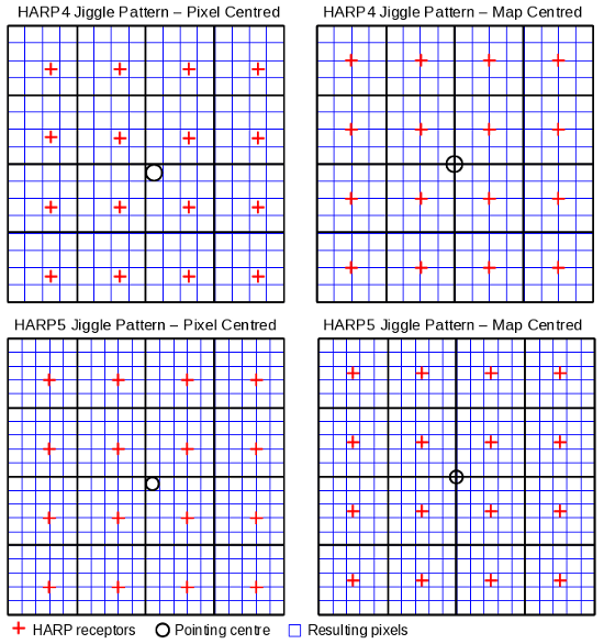
Each of these patterns can be pixel-centered, where the target co-ordinates fall on one of the central four pixels, or map-centered where the target co-ordinates lie at the centre of the map between the four central pixels. See Figure 3.3 for an illustration of the different jiggle patterns. Although designed for HARP this mode can be used with the single-element receivers. |
| Raster | Raster mapping, or scan mapping, is designed for mapping large areas with maximum efficiency. The telescope continuously takes data while scanning across the source. When HARP is used for raster mapping the array is rotated 14.°04 to the direction of the scan in order to give a fully sampled map with 7.″3 pixels. This will result in jagged edges to your reduced map which you may wish to trim. It is common when using HARP to repeat the map scanning along the other axis to give a ‘basket-weave’ pair of maps. Each one of the pair will appear as an individual observation. The right-hand panel of Figure 3.2 shows a HARP raster map. |
| Position-switch |
In position-switch (PSSW) mode, the whole telescope moves off source and on to the reference position. This allows a large offset to the reference position, useful in crowded environments such as the Galactic Plane. The main disadvantage is that it takes a longer time resulting in less-accurate sky subtraction or non-flat baselines. |
|---|---|
| Beam-switch | In beam-switch (BSW) mode, the secondary mirror chops onto the reference position. This results in fast and accurate sky subtraction but it is limited to targets which have a blank reference position within 180′′(the maximum chop distance of the SMU). |
| Frequency-switch | In frequency-switch (FSW) mode the telescope does not move but the centre of the spectral band is shifted, typically by 8 or 16 MHz, to a line-free region of the spectrum. It is very efficient with no off-source time and can be useful when no emission-free reference position can be found. |
SKYREFX and SKYREFY with
respect to the base position given by BASEC1 and BASEC2, respectively. Details may be found in
SUN/259.
Subsystems are normally arranged to cover different spectral lines and would be processed independently. However, there is also a mode in which the subsystems overlap in frequency, called hybrid. Such data are combined to yield a broader spectral coverage, say where there multiple lines in proximity. The number of subsystems is up to a maximum of four.