Processing math: 100%
Chapter 5
The ACSIS Pipeline
The Orac-dr pipeline [4] is a generic automated data reduction pipeline that can process your raw JCMT data
and return advanced data products: baselined single observation cubes, mosaicked and co-added cubes,
moments map and clump catalogues. [15]
It has advanced algorithms for the common routines such as baseline subtraction. The data processing is
performed using standard Kappa, Smurf, and Cupid applications, the main ones of which are described in later
chapters.
5.1 Recipes and primitives
Reduction recipes in Orac-dr consist of a series of stand-alone processes, known as primitives.
These primitives are linked together to form data reduction recipes. Each primitive can be fed
different input data depending on the nature of the recipe in question and may sometimes be omitted
altogether.
There are four main science recipes available, each tailored to different type of observation:
A summary of these recipes is given below.
|
|
|
| RECIPE | DESCRIPTION OF EMISSION | BASELINE METHOD |
|
|
|
| NARROWLINE | One or more narrow lines are expected
across the band. Select this recipe if
the expected lines are less than about
8 km s−1 wide. | Smoothing:
spatial =
5×5
pixels
frequency = 10 channels |
|
|
|
| BROADLINE | This recipe is designed for wide lines that
extend over a large fraction of the band.
The line is typically too weak to see in
a single observation so a pre-determined
baseline window and linear baselines are used. | Uses the outer 10% of each
end of the spectra to fit a
single-order polynomial. |
|
|
|
| GRADIENT | Typically one moderately wide line is
expected, for which the center velocity varies
significantly across the field. The baseline
window changes across the field. Nearby
galaxies often fall in this category. The
expected lines should be wider than about
8 km s−1 and
probably not wider than 20% of the available
bandwidth | Smoothing:
spatial =
3×3
pixels
frequency = 25 channels |
|
|
|
| LINEFOREST | A forest of lines is expected across the band.
Bright, nearby star-formation sources may fall
in this category. This recipe also creates a
separate moments map for each line (as defined
by the parameter PER_LINE). | Smoothing:
spatial = none
frequency = 10 channels |
|
|
|
| |
There are also variants of the recipes with the following suffixes.
| _POL | polarimetry |
| _QL | Quick Look which merely runs makecube to turn the raw
time-series spectra into a spectral cube for display during data
acquisition. |
| _SUMMIT | A limited reduction to keep pace with data acquisition at the
JCMT. It excludes any bad spectra rejection, quality assurance, or
iterative baseline determination. |
| |
5.2 The workflow
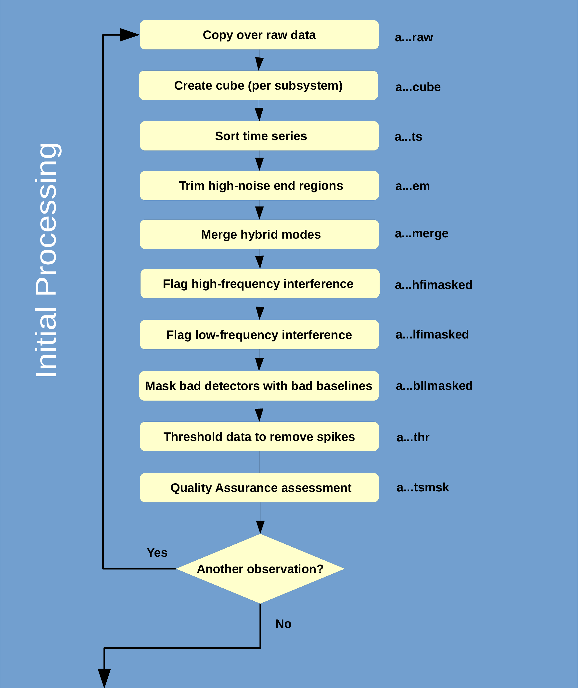
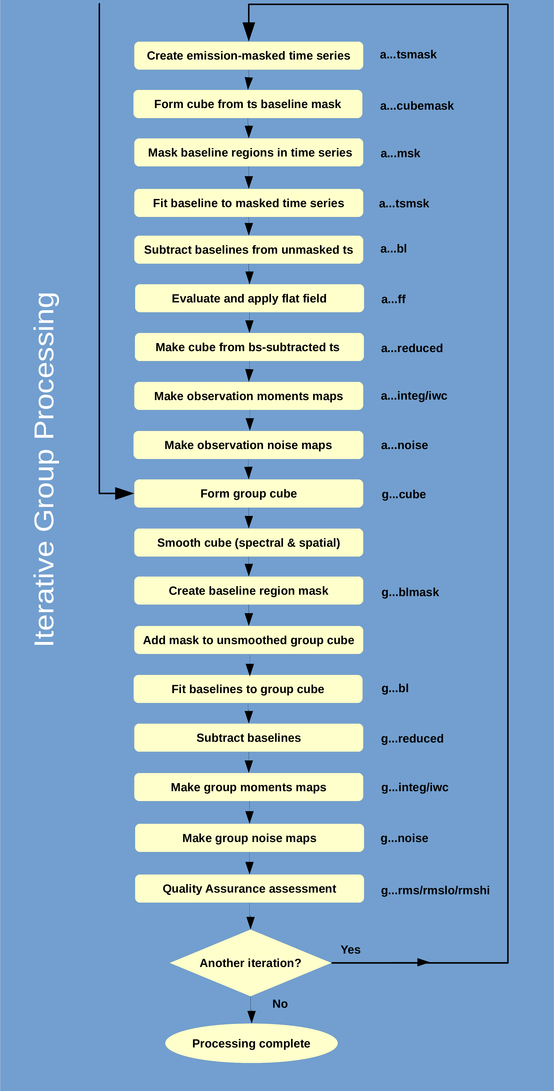
You can follow this commentary via the flow chart in Figure 5.1.
Two notations are used in the following list:
∙ a_cube to mean the regridded cube of a single observation.
∙ g_cube to mean the group cube which is a co-add of all the a_cube files.
Note that the pipeline will co-add data into a group file whenever it encounters observations with identical LO
frequencies, base positions and bandwidths. You can also force a set of observations, such as ones of the same
object taken on different nights, to be regarded as a single group to be combined via the oracdr -onegroup
command-line option.
-
(1)
- The raw data are copied to the local directory. Typically, subsystems are treated as individual and
separate observations by Orac-dr except for hybrid-mode observations.
-
(2)
- Because data acquisition is asynchronous, time slices are not necessarily written in sequential
order. The next step sort the time-series data into time order. This makes it easier to search for
intermittent bad data.
-
(3)
- The noisy ends of the spectral band dwarf most astronomical signal, and hence are removed as
follows. The spectra are collapsed along the receptor using the ‘sigma’ estimator to form a single
spectrum. A constant value background is then fit to the resulting spectrum. The fitting regions are
used to determine where the spectrum gets noisier (i.e. higher RMS values in the RMS spectrum).
These high-noise regions are then trimmed from the ends in the frequency axis. There is also an
alternative to trim specified percentages through the
TRIM_ recipe parameters (see Table G.2).
-
(4)
- The DC-level offset between corresponding sub-band observations is determined using the
median of all the spectra. The DC offset is then subtracted from the sub-band spectra, and the
resulting sub-band spectra are mosaicked together to form single time-series cube.
-
(5)
- Regions or individual spectra containing high- and low-frequency interference from local sources
are identified and flagged. Bad detectors are identified by comparing the deviation from linearity
of each detector’s baseline.
-
(6)
- Strong spikes (±150)
are replaced by bad values.
-
(7)
- Quality assurance checks are run on the raw cubes. See Appendix H for a description of the checks
performed. Any time-slices failing any of these checks gets flagged as bad and are not included in
the group co-add that follows.
-
(8)
- Once all the raw observations have undergone the initial processing, the individual time-series
files are combined to form a g_cube.
-
(9)
- The g_cube is smoothed by an amount specified by the particular science recipe being used. See
Section 5.1 for details on the different recipes.
-
(10)
- mfittrend is run to find the baseline regions on the smoothed g_cube. The ranges are determined
automatically by setting
auto=true. A baseline mask is written out.
-
(11)
- The baseline mask is then applied to the unsmoothed g_cube and mfittrend is re-run. This time
however, the emission regions have been masked out, so all remaining data are included in the fit
by setting
auto=false. The resulting baseline is subtracted.
-
(12)
- Moments maps and noise maps are made from the baseline-subtracted g_cube.
-
(13)
- If another iteration is required, continue to Step (14). If not, the processing is complete.
-
(14)
- The baseline mask is converted back to the time series with unmakecube. There it is applied to
the time-series data for each observation.
-
(15)
- A baseline is fit to the masked time-series data using mfittrend and the result is subtracted from
the unmasked time-series data. This can be a higher-order polynomial (up to 15th
order), although a linear fit is often used.
-
(16)
- A flat field, i.e. the relative responsivities of the detectors, is optionally created and applied. It
involes making cubes for each each receptor combining all observations on a given date to improve
the accuracy. There is a choice of analysis methods, but an iterative approach of thresholding—to
exclude the noisy baseline that would dilute the comparisons—worked best on most suitable
observations. Those with low signal-to-noise or signal only originating in a small percentage of the
area mapped are not amenable to determining the receptor-to-receptor responses. (See Table G.5).
-
(17)
- An a_cube is made from the baseline subtracted data for each observation.
-
(18)
- The individual baseline-subtracted time series are combined to make a new g_cube.
-
(19)
- Return to Step (9).
Copyright © 2015-2021 Science and Technology Facilities Council,
& East Asian Observatory


