In this section each of the basic steps in the longslit spectral data reduction procedure are described. Many of the initial steps are similar to those for 1-D data and reference will be made to those sections with notes for any slight differences. Later steps do become 2-D data specific.
Examples of practical techniques using these ideas are to be found in §7.
The essential basic difference with 2-D data is that we are not looking to extract a region of the CCD frame into a single spectrum but wish to preserve the spatial direction in order to study changes in the spectrum with position.
Given this, the initial image preparation is the same as for 1-D data which is described in §4.1 and §4.5.
The order in which 2-D data is calibrated is different to that for 1-D data. Many of the tasks in processing the data (e.g. background sky emission line subtraction) require the 2-D frame to be correctly oriented with spatial and dispersion axes perpendicular.
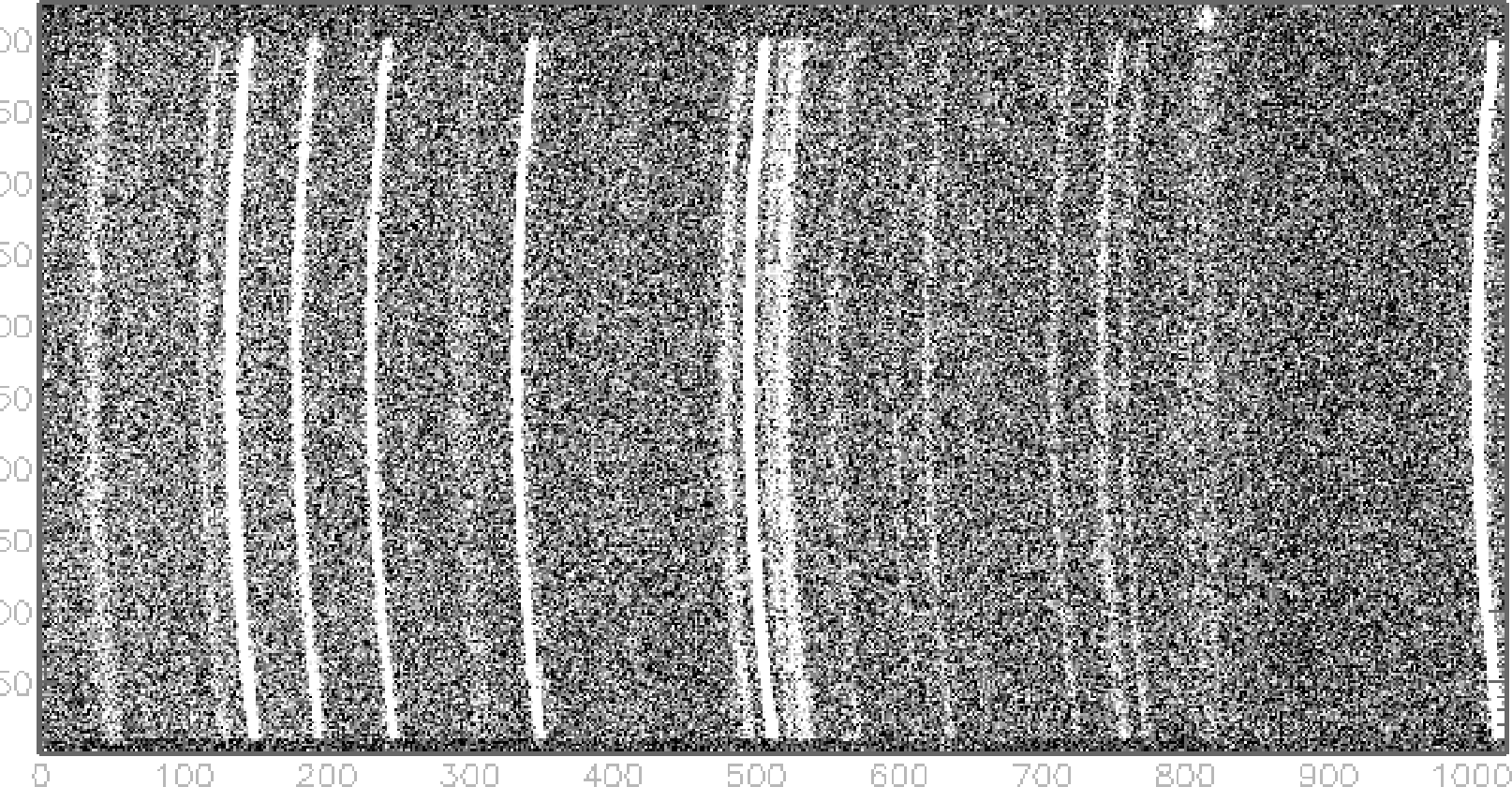
As can be seen in the example arc line image (see Figure 13,page 60, for an example) the lines have a definite curvature along the spatial axis. This is due to the different path lengths the light takes through the optics along the slit. Correcting for this is carried out along with wavelength calibration.
The process of wavelength calibration along the dispersion axis also allows us to correct for the geometric curvature of the frame described above.
The wavelength calibration works in the same way as described for 1-D spectra, matching the wavelengths of known arc lines to the pixel values for the centres of the lines and performing a polynomial fit to the data. Before this can be done we must calculate the curvature of the arc lines on the frame in order to straighten them.
Both of these tasks are typically done by the fitting of Gaussian functions to each arc line profile for each cross-section of the frame. These then give the centre of each arc line for each cross-section which can then be fitted by a polynomial along the arc line. A polynomial matching pixel and wavelength values along the dispersion axis can then be fitted.
For 2-D frames these fits are output in an .iar file, which contains the polynomial coefficients. These can then be used by other programs to ’scrunch’ the data, in other words to resample the data correcting the distortions and calibrating the wavelength axis.
As with 1-D spectra it is important to use arc lines which enable a sensible polynomial fit to be made, i.e. well spaced over the whole of the CCD. Similarly, as low an order polynomial as sensibly fits the data should be used to prevent large errors being generated at the ends of the dispersion axis.
With the solution calculated for the calibration of the 2-D frame the next stage is to apply this to the data. This process is called scrunching.
The program (e.g. iscrunch in figaro) will take your .iar file containing the solution and a data frame and apply the corrections and calibration to it. This will involve re-binning the data and adding a new wavelength axis.
It can also be a useful test to scrunch the original arc frame, which should result in a set of perfectly straight arc lines.
A slightly more advanced program (iscruni in figaro) will allow you to use two .iar files and use the average values when calibrating the data. This is useful for long data exposures where arcs may show a shift from arc line images taken before and after the data.
Flux calibration works in much the same way as for 1-D spectra, see §4.8.1.
The only difference comes when applying the calibration to the data when each row of the 2-D frame is calibrated rather than a simple spectrum.