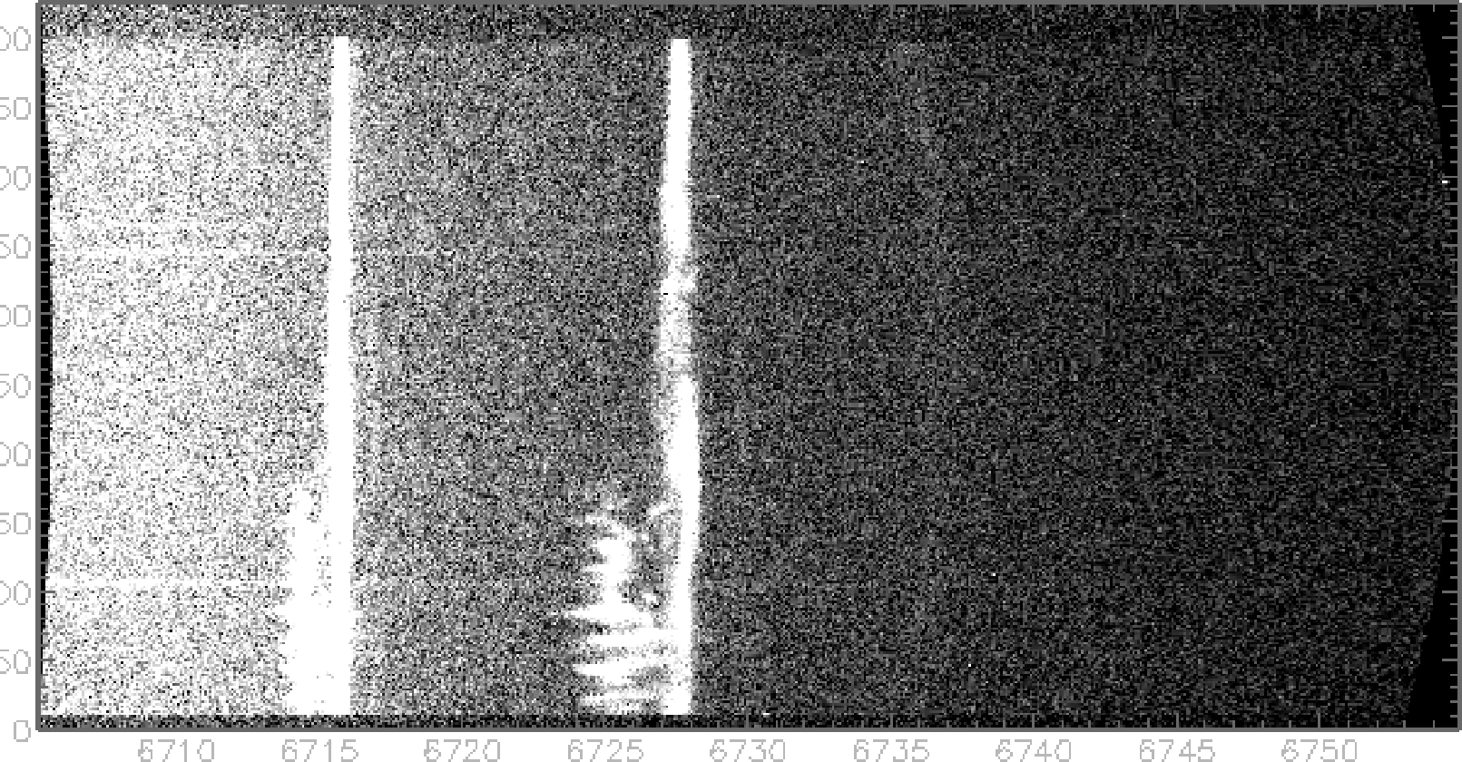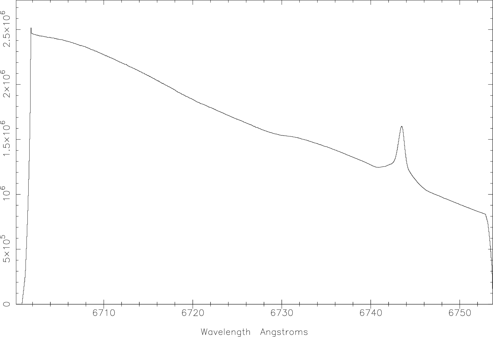
Figure 14: An arc line spectrum with lines selected between the tram-lines.
As there may be readers who have come to this section without reading the worked 1-D example I will reiterate a number of instructions. If you are familiar with the early steps please feel free to skip on.
Before you start the extraction you will have to do the detector-specific preparation of your data (most likely to remove CCD-related effects). If you have not done this, refer to §4.1 for an outline of the procedure, and §1.2 for pointers to documentation of the process.
The first thing you need to do (if you’ve managed to prepare your CCD data you will most likely know this already, but…) is to run the Starlink setup. Normally Starlink software is installed in the /star directory and the commands you must execute are:
If your Starlink software is installed somewhere else, then modify the commands appropriately. Most people include these lines in their shell login file (.login in your home directory).
Once you have done the Starlink ‘login’ you can initialise for any of the major packages simply by typing their names. For example, we are going to use figaro[18], kappa[8] and twodspec[23] and so get a display something like:
We can now use figaro, kappa and twodspec commands.
As with the 1-D example, you might like to take a copy of the example data which comes with this document when installed as part of the Starlink document set. You will find the files in the directory
Create an empty directory and enter it using cd. To copy the test data type the command
You will then find you have these data files in your directory:
| File | Description |
object2d.sdf | Frame with the object spectrum |
arcframe2d.sdf | Frame with a wavelength-reference arc |
quartz2dscrun.sdf | Frame with a quartz lamp flat field |
At this stage it is assumed that the image files have been de-biased and cosmic ray cleaned.
The first thing to do is to put the image frames on display for inspection. This can be done using kappa display:
This shows the data frame with two emission lines, in this case from the Honeycomb Nebula in the Large Magellanic Cloud. (see Figure 2, page 11).
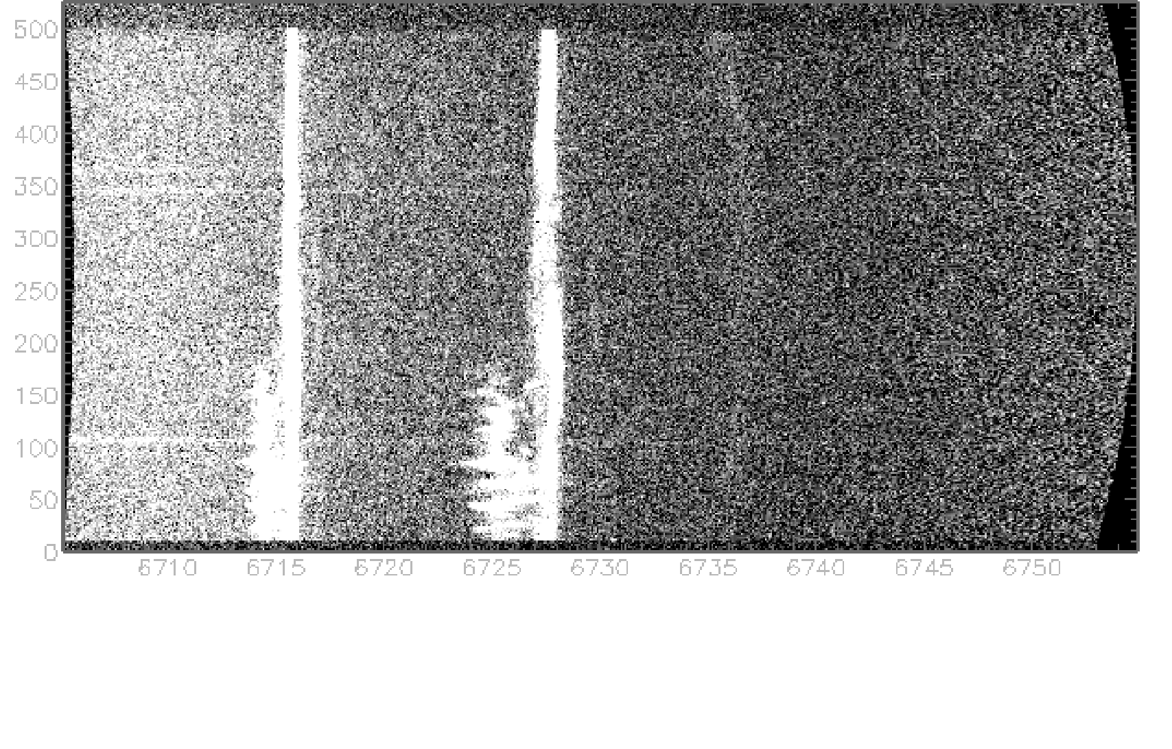
The arc line image can be shown using:
The curvature of the arc lines, which we wish to correct, is obvious (see Figure 13, page 60.
There are three key elements to the inspection of the images at this stage,
These frames are correctly rotated (i.e. have the wavelength axis parallel to the x-axis) and have wavelength increasing to the right. If this is not the case with your data, methods for correcting this were detailed previously in §5.2.
With the arc line image displayed we can carry out the third item mentioned above, noting the range of y-axis values the arc lines extend over. To do this we can use the kappa cursor command:
The cursor should then be placed at each end of an arc line and the left mouse button clicked. This will report the coordinates of the point in the terminal window. When this has been done click the right mouse button to exit.
When I did this I obtained these values:
So we have a range of 13 to 493 in the y-axis.
We can now go on to the fitting of these arc lines.
To carry out the fitting we use the twodspec command arc2d. This program provides a number of
menus and interactive displays and will be described in the text.
We wish to carry out a new identification of the arc lines so type new and press return. The program
will ask for confirmation of this action, enter y to the questions.
This question asks for the number of arc lines you wish to use. Ideally you would like a number of lines spread evenly over the CCD array. As the resulting fits are typically 3rd order or lower then 5 lines is a reasonable default. Press return.
In order to identify the arc lines we have to select them interactively. These question ask for the range of y-axis values over which to extract a spectrum for this identification. Simply enter the values which we found using the cursor earlier.
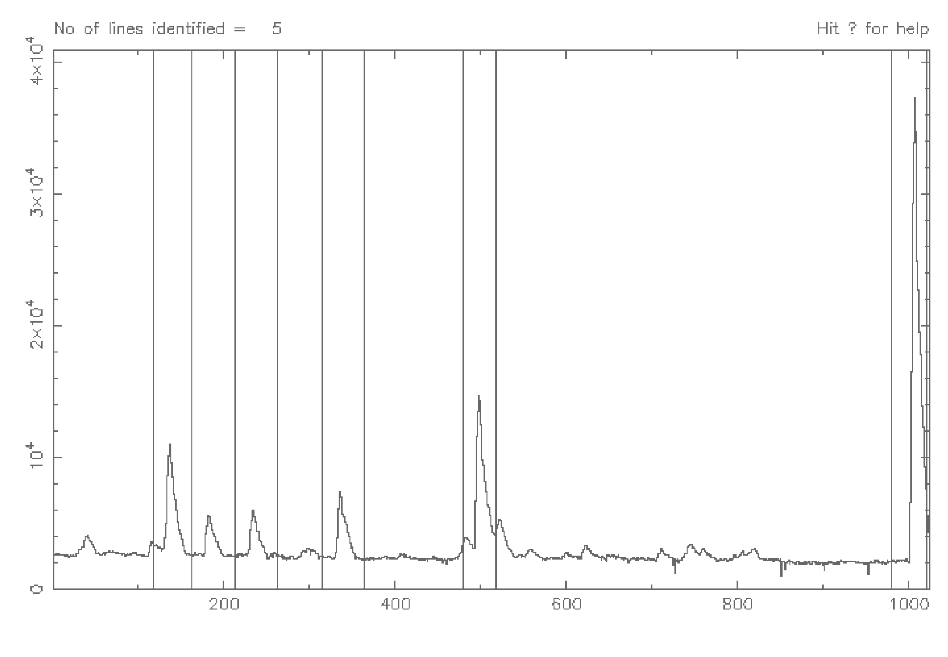
At this point the extracted spectrum will be displayed on the graphics window. You will see that the lines are quite broad as we have summed the data over a range in the y-axis and hence in curvature of the line.
The lines are then selected using the mouse, going from left to right across the spectrum in increasing wavelength. To select the lines to be used the left mouse button is clicked to the left and right of the arc line to mark tramlines. Only one arc line should lie within the tramlines and there should be some continuum left on each side of the line in order to fit a good baseline (see Figure 14, page 67)
Once you have marked out each of the arc lines you wish to use press e to exit this stage. You are now
given the option of selecting a line list, simply a text file of known lines for particular arc lamps or
emission lines. These can be used as a reference when identifying the selected lines. In this case the arc
was a Thorium Argon lamp for which a list is not available. The lines will then have to be identified
using an arc line catalogue.
So we can type ok at this prompt.
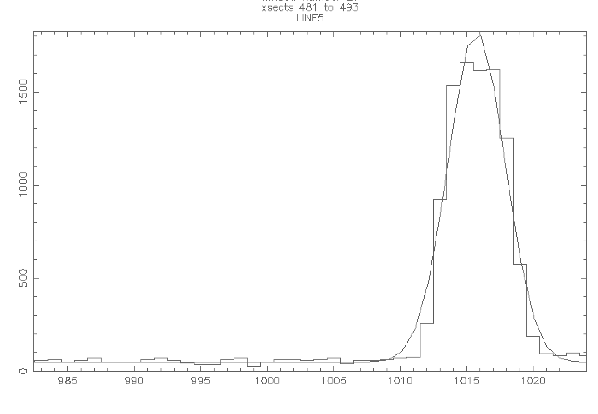
The program now displays the first selected line in more detail and prompts you for an identification on the terminal screen.
As we have found the arc line pattern in the catalogue we can enter the known wavelengths for each arc line. The first line has a wavelength of 6708.97 angstroms and so we enter
and then confirm this is correct.
The second line is now displayed and we similarly enter the wavelength for this line. The wavelengths for the five lines marked in Figure 14) are:
After this the program will display the entered list of identifications for you to check. Enter no to ’edit line list’ to reach the main menu:
So we now have the lines identified with their wavelengths. The next stage is to fit a Gaussian to each arc line for each row of the image. The centres of these Gaussians will then be used to calculate the corrections required.
Fitting these Gaussians is selected by entering gaus at the main menu prompt. Again we are asked for
the limits over which rows the program should try and fit Gaussians to the data. These should be the
same limits as you entered earlier, and the program will suggest these values as defaults. The next
question regards the blocking factor. There is cost in processing time depending on how many
Gaussians you fit and one way to reduce this is to add a block of rows together. Typically a blocking
factor of 4 percent of the total number of rows is reasonable, so for our case a value of
18 pixels. This value is not crucial, so long as it is not larger then any obvious distortion
in the arc line across the CCD. Blocking also brings a benefit in that it will increase the
signal to noise ratio of the data and is often essential in getting a good fit to low signal arc
lines.
Enter 18 and press return. The next question asks if you wish to see the Gaussian fits as they are
carried out. If this is the first time you have done this you may want to say yes, but experienced users
might say no as typically the fits are not very exciting and do take some time to go through. An
example Gaussian fit is shown in Figure 15, page 71.
After this has been completed you are returned to the main menu. With the Gaussians fitted the next stage is to calculate the straightening of the arc lines. This is done by fitting a polynomial to the centres of the Gaussians for each arc line in the y-axis direction.
Enter poly and press return. Enter no at the next prompt regarding errors and no to the next
question regarding weights as we wish to fit the polynomials solely on the centres of the
Gaussians.
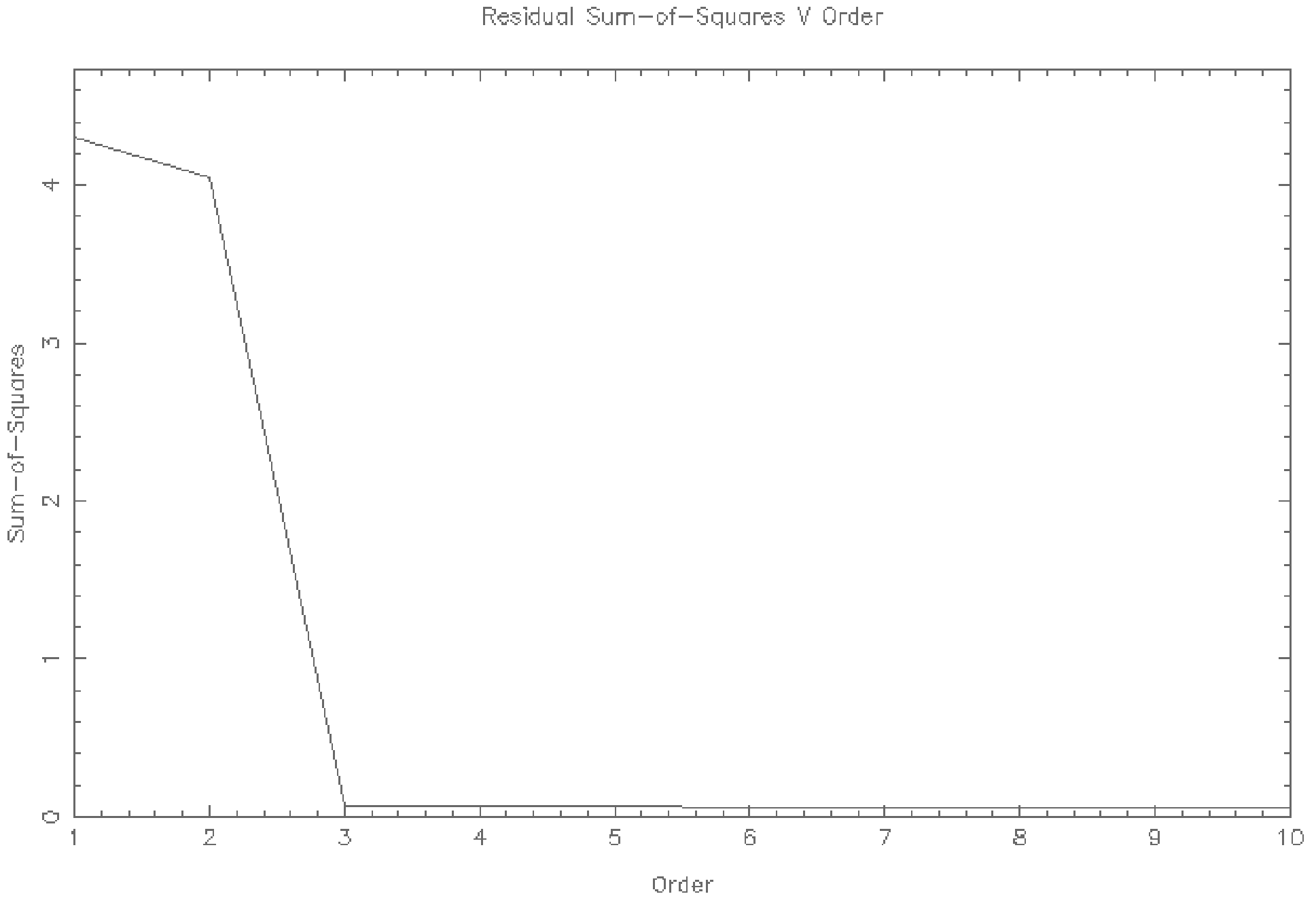
Now displayed is a plot showing the residual sum of squares of the polynomial fit to the fitted centres for increasing polynomial order. As can be seen in Figure 16, page 74, the third order fit looks to be a good one.
If you reply yes to the request to go on to next plot you will be shown the residuals
for a first order polynomial. Press return again will show the second order fit and
so on. Looking at the residuals to the third order fit we can see they are less than
±0.1 pixels.
At this display enter no to the request to see further orders.
The program then asks for the order you wish to use:
Enter 3 here and press return.
Now the data points and polynomial fit are displayed for the first arc line (or tooth as it is described here). Again we can continue to look at the data and fit for each of the arc lines.
When you reach the last line or type no earlier you are asked if you wish to produce a hard copy
of the plots. For now select no and the program will ask if you want to accept the fitted
polynomials:
Enter accept to return to the main menu.
With the straightening of the arc lines calculated the next step is to calibrate the wavelength
dispersion axis. From the main menu enter disp to select the ’Evaluate dispersion relation’
option.
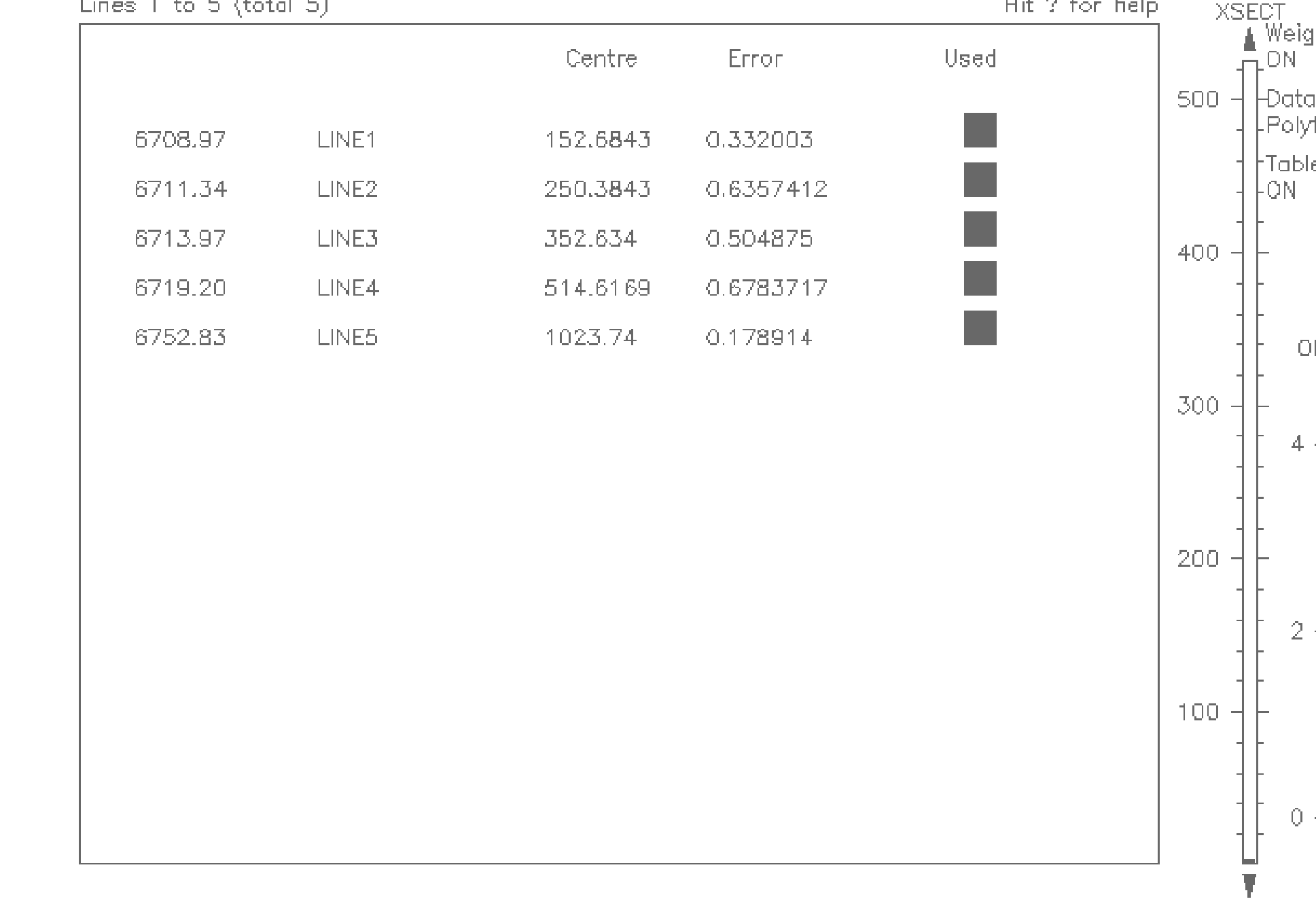
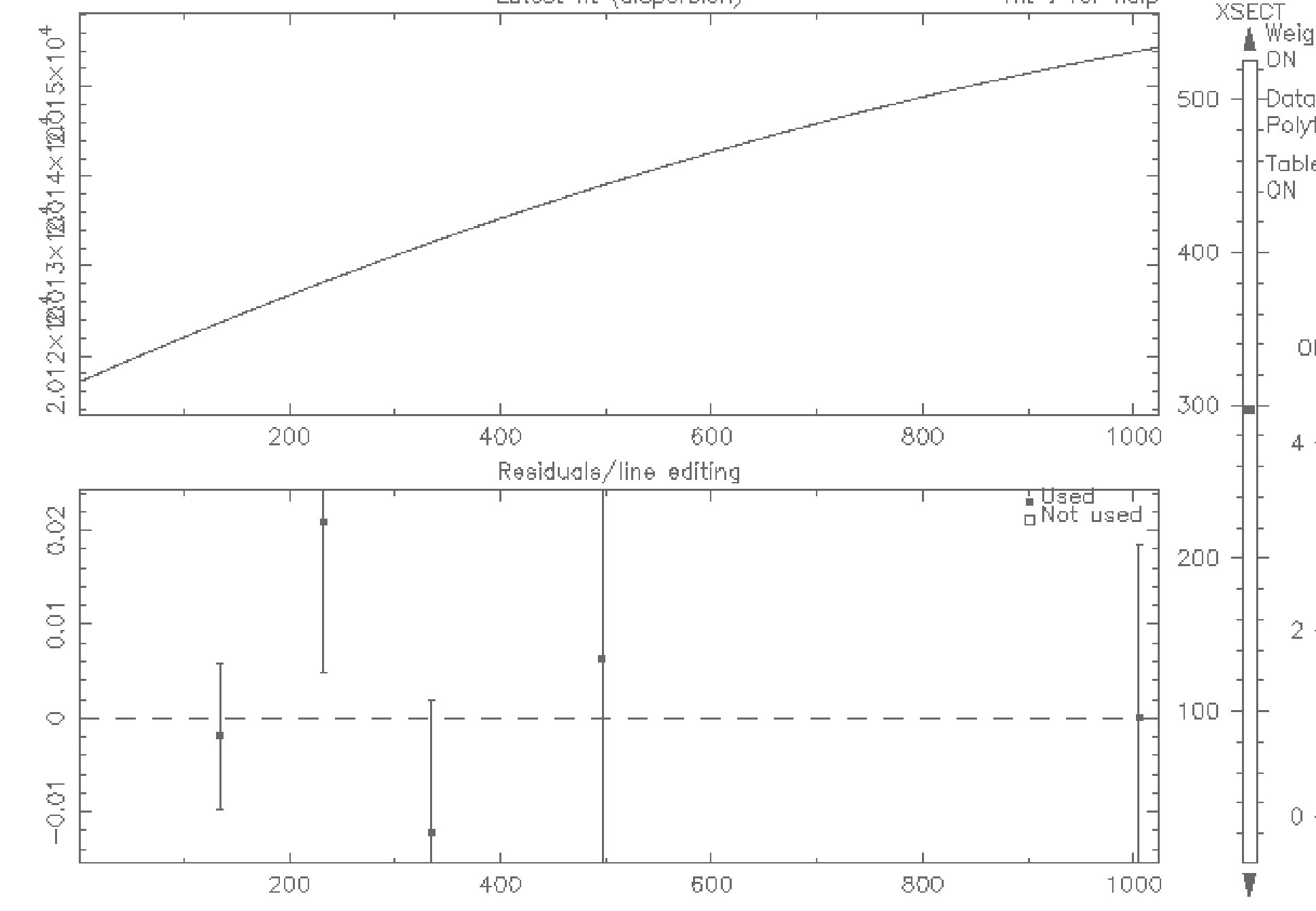
The dispersion screen is then shown on the xwindows display (see Figure 17, page 77,). The arc lines are listed with boxes to toggle the use of that line in the calculations.
On the far right of the display is a selector for the order of fit to be used and then the y-axis (or X-section) number to perform the fit at.
In this case we shall use a 3rd order fit (which should already be selected) and to perform the fit at a y-axis value of around 300. You will need to click next to 300 in the slider at the right hand side of the display. The marker should then be shown at 300.
Then carry out the fit, which solves the non-linear pixel value to wavelength value relation, press f
while the cursor is in the main panel.
The program then displays the polynomial used for the fit in the upper panel and the residuals in the lower panel. Residuals of less than ±0.05 are usual for a good fit. See Figure 18, page 80, for an example fit.
We could then go on to try a 2nd order polynomial fit - select order two by clicking the order selector
at the right of the screen and press f again. You can see then residuals are now around
±0.5.
Select order 3 again and refit the data (press f again).
When you are happy you press a to accept the fit. Control now reverts to the terminal window
where you can opt to see tables of the fit results. Enter no to this and the next question
regarding copying fits from one line to another. You will be asked to confirm the fits are
ok.
When the fits are completed a line looking like:
will have been displayed. These numbers are important and are used in the scrunching step to come.
The program then returns to the main menu and reports the writing of an .iar file which contains our polynomial fits.
We can now select exit to leave the program.
The .iar file generated is a simple ascii file and can be looked at with more:
The .iar file can be used by the figaro iscrunch program in order to correct and calibrate your data files:
You will then be asked for the name of the .iar file:
enter arcframe2d.
The next question asks how many bins (pixels) you would like your new image to have. The simplest
answer is to keep the same number of pixels that you had in your original image, hence for this file
enter 1024
The next question ask if you want to sample your data in logarithmic bins, enter false.
You will now be asked for the start and end wavelengths of your data, use the numbers noted earlier after the dispersion had been calculated.
The next question asks if the data should be treated as a flux per unit wavelength. Typically for data
from spectrometers the answer to this is false.
Reply true to use quadratic interpolation for the data at the next question.
The final question asks for the output filename, e.g. object2dscrunch:
We can now view this scrunched file using:
which should look something like Figure 19, page 84.
A further check on the process is to scrunch the arc frame, in order to check that the arc lines do indeed come out perfectly straight.
To remove the wavelength dependent sensitivity or blaze from the data we need to use a quartz flat. The file quartz2dscrunch.sdf is a ready scrunched quartz lamp image.
The bright line towards the right of the image is a ghost. We wish to generate a smooth fit to the quartz lamp and the easiest way of doing this is to add together the rows to form a single spectrum. We use the values for the range in y-axis obtained earlier from measuring the arc lines.
This generates a spectrum quartzspec.sdf which we can view with
As can be seen in Figure 20, page 87, this spectrum has zero values at each end and the ghost line appears superimposed on the quartz lamp continuum. In order to remove these effects and obtain just the continuum we fit a polynomial curve to the data. We use the figaro cfit command:
Use the cursor and mark points (using the a key) along the spectrum, including points at the start and
end where we have no data and ignoring the ghost line. When you have finished this press x the exit.
The fitted line is then drawn over the spectrum.
We can view this on its own with
We now have a smooth spectrum to divide into our data but before we do this one further stage is to normalize this curve. To do this we need to find the mean value for the quartzfit spectrum:
For my fitted spectrum this gave these results:
The key number is the pixel mean value of 1663793, which we will divide the spectrum with to give a mean value of 1.
We can now finally use this normalised spectrum to correct our observed data using the figaro isxdiv command:
This command divides the quartz spectrum into each row of our data frame to produce the quartz
corrected file object2dscrunchnorm.sdf (see Figure 21, page 90.
) with:
With the data calibrated you have now completed the data reduction of a 2-D longslit spectral array. For analysis of this data you may want to use the twodspec[23] longslit package or dipso[11].