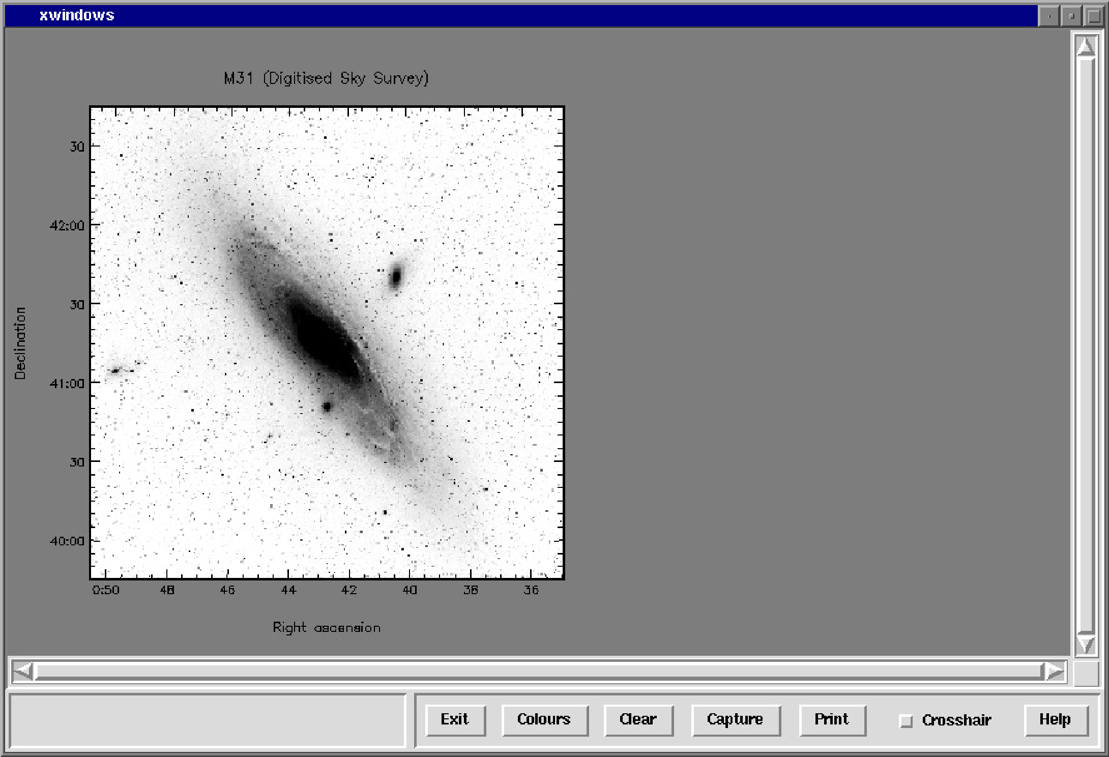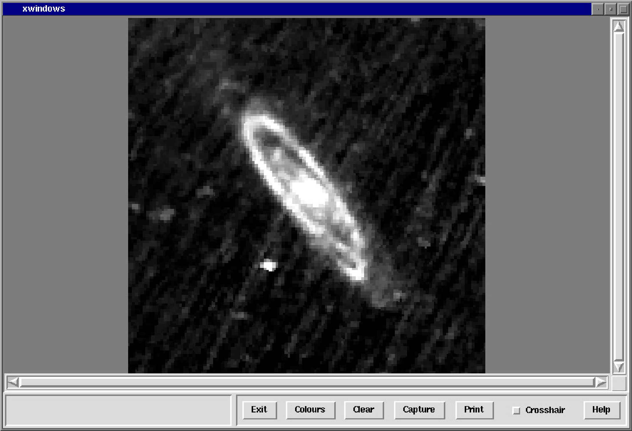
Figure 1: An IRAS 12 μm
image of M31 displayed in the middle of the BASE picture.
Have you ever been in a situation where you would like an application to know about graphics drawn by some other programme? For instance, you display an image of the sky, then later you want to obtain the co-ordinates of the stars within the image via the cursor. There are two main approaches to achieving this functionality. The first is to duplicate the display code in the CURSOR application. This is wasteful and inflexible. The second is to store information about ‘pictures’ in a database that can be accessed by subsequent graphics programmes. This is the technique used by Kappa.
Each graphics application that creates a display on a graphics device, also stores information describing the display in the graphics database. This is a file, which usually resides in the user’s home directory, and is often referred to as the AGI database.10 Displays are described in terms of pictures. A picture is basically a rectangular area on the graphics device within which an application produces graphical output. Each time an application creates a picture, the dimensions and position of the picture (together with other ancillary information) are stored in the graphics database. Subsequent applications can then read this information back from the database, and use it (for instance) to align new graphics with previously displayed graphics.
The best way to demonstrate the use of the graphics database is to give some illustrated examples.
The following examples assume that Kappa is loaded and the graphics device—an X-window
containing a plotting area of 850 by 500 pixels—is available. To create such a window use the xmake
(SUN/130) command:
This command limits the number of colours used by the X-window to 64. It is usually a good idea to be sparing with X-window colours. Creating X-windows with too many colours can restrict the availability of colours for other X applications.
First of all we make the X-window the current graphics device (as described in in global device names.) This selection will remain in force until changed. The following command would not be necessary if the global parameter already had this value:
Next we shall clear the X-window, and empty the graphics database of xwindows pictures (pictures relating to other graphics devices are retained):
The display is now clear, but one picture remains in the graphics database; this is the BASE picture and corresponds to the entire plotting area. To understand why this BASE picture is required we need to introduce the idea of the current picture.
At any time, one of the pictures stored within the graphics database is nominated as the current picture. All graphical applications are written so that the graphical output that they create is scaled to fit within the current picture. Thus, the plotting area used by a graphics application can be controlled by selecting a suitable current picture before running the application. Since we have just cleared the database, the only picture remaining is the BASE picture, which consequently becomes the current picture. This allows subsequent applications to draw in any part of the plotting area.
We now load a grey-scale colour table into the X-windows and display an IRAS 12 μm image of M31. The pixel values are scaled so that 10% of the pixels appear as pure black, and 1% appear as pure white. We ensure that no annotated axes are produced (this will result in the image being a little larger since no margins need to be left for the axes):
The X-window should now look like Figure 1. The application has displayed the image in the middle of the current picture (the BASE picture), and has made it as large as possible, subject to the constraints that it must lie entirely within the current picture. Note, as with many IRAS images, equatorial north is downwards in this image
Let’s now use the PICLIST command to look at the contents of the graphics database (press return in response for the prompt for Parameter PICNUM):
This shows us that there are now two pictures in the database, listed in the order in which they were
created. The current picture is still the base picture, as indicated by the letter C at the left of the line
describing picture number 1. The second picture was created by the Kappa application DISPLAY, and
has the name DATA, indicating that it contains a representation of a set of data values. DATA is one of
four standard picture names. BASE is another of these standard names. We shall come
across the other two shortly. The PICLIST application allows you to select a new current
picture by supplying a picture number in response to the prompt for parameter PICNUM.
Accepting the null default by pressing return causes the current picture on entry to be
retained.
The above use of DISPLAY illustrates an important rule regarding the behaviour of most graphical applications; the current picture is not changed by applications that produce graphical output.11 If it were not for this rule, pictures would become progressively smaller, vanishing into the distance, since new pictures cannot be drawn outside the current picture.
We will now display an optical image of M31. This time we will arrange for it to be placed towards the left hand side of the X-window. To do this, we first clear the whole X-window and graphics database using GDCLEAR:
We now create a new picture using the PICDEF command (note, the "\" characters are needed to prevent the UNIX shell interpreting the square bracket characters):
The MODE parameter specifies the position of the new picture within the BASE picture; in this case
"cl" indicates that the new picture is to be centred ("c") vertically within the BASE picture and placed
at the left ("l") hand edge. The FRACTION parameter specifies the dimensions of the picture; the first
value (0.6) gives the horizontal size of the picture as a fraction of the horizontal size of the BASE
picture, and the second value (1.0) gives the vertical size of the picture as a fraction of the vertical size
of the BASE picture. Thus, the new picture is just over half the width of the BASE picture, and is the
full height of the BASE picture. The OUTLINE parameter specifies whether a box should be drawn
on the screen showing the outline of the new picture. In this case we switch this option
off.
If we run PICLIST again, we get:
The picture created earlier by DISPLAY was deleted when we ran GDCLEAR. The BASE picture is still
there (of course), and we also have the picture created by PICDEF. This is a FRAME picture, another of
the four standard picture names. A FRAME picture acts as a ‘frame’ for other pictures. A FRAME
picture can itself contain other nested FRAME pictures, together with DATA and KEY pictures. The
picture created by PICDEF is the current picture (indicated by the letter C again), and so subsequent
graphics applications will arrange for any pictures they create to fall entirely within this FRAME
picture.
Now display the image, this time including annotated axes around the edges.12 DISPLAY will ensure that all its output (both the image and the axis annotation) fall within the current picture (i.e. the picture created by PICDEF above). We scale the pixel values to produce a negative image in which 1% of the pixels appear black and 30% appear white:
The X-window should now look like Figure 2. We can use PICLIST again to list the pictures stored in the database:
There are four pictures this time; the BASE picture, the picture created by PICDEF (number 2), and two pictures created by DISPLAY (numbers 3 and 4). Picture number 2 was made the current picture by PICDEF and as explained above, DISPLAY did not change this. DISPLAY creates two pictures, one (the DATA picture) containing just the image area itself, and another (the FRAME picture) to act as a frame for the DATA picture and the annotated axes.
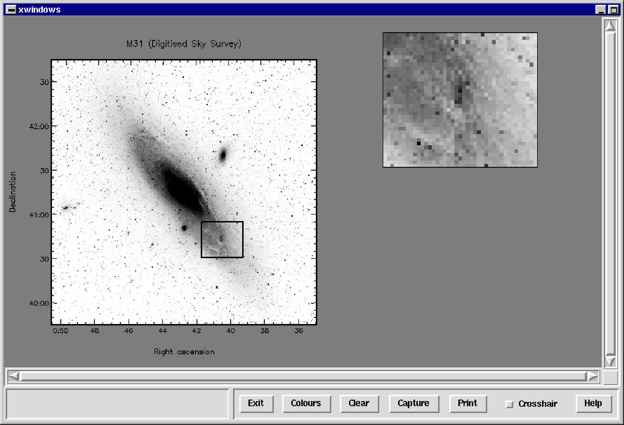
Let’s say you wanted to display an enlarged sub-section of the image in the top-right corner of the X-window. First, you need to decide on the bounds of the sub-section to be displayed. Here, we use a graphics cursor to indicate the bottom left and top-right corners of a box enclosing the required area. Click the left mouse button at the bottom left and top right corners of a box enclosing the required sub-section of the image:
The box I selected is indicated in Figure 3.
When an application such as DISPLAY produces a DATA picture containing a representation of an
NDF, it saves a copy of the NDF’s WCS component (which contains co-ordinate Frame information)
with the DATA picture in the graphics database. When CURSOR subsequently reports a position, it
uses this saved WCS information to convert the graphics co-ordinates at the cursor into any of the
available co-ordinate Frames. By default, CURSOR reports positions in the co-ordinate Frame that was
current when the NDF was displayed (RA/DEC in this case), but other co-ordinate Frames may be
requested using the FRAME parameter (e.g. FRAME=PIXEL displays pixel co-ordinates). In
addition to the co-ordinate Frames inherited from the NDF, there are also four extra Frames
available.
Going through the parameters supplied to the above CURSOR command, the first one
(SHOWPIXEL) causes the pixel co-ordinates at each selected position to be displayed,
in addition to the co-ordinates selected using Parameter FRAME (which defaults in this
case to RA/DEC since FRAME was not specified). For instance, the first position is at a
right ascension of 0h41m33.5s and a declination of +40°33′1′′, and has pixel co-ordinates
(172.4,78.2).13
The second parameter (PLOT=BOX) causes a box to be drawn on the screen between each pair of
positions. There are several other allowed values for the PLOT parameter, which mark
the positions in different ways (markers, poly-lines, chains, text, etc.). The last parameter
(MAXPOS=2) is purely a convenience, and causes the application to terminate when two positions
have been supplied. Without this, you would need to press the right mouse button once
the two positions had been given to indicate that you do not want to supply any more
positions.
We now need to create a new FRAME picture to contain the magnified image section. We have seen how PICDEF can be used to create a FRAME picture of a given size at a given position within the BASE picture, but there are also several other ways in which PICDEF can be used. Here, we use PICDEF in ‘cursor’ mode; the bottom left and top-right corners of the new picture are specified by pointing and clicking with the mouse.14 We use this mode to create a new FRAME picture occupying the area to the top right of the existing image:
The co-ordinates displayed by PICDEF are BASEPIC co-ordinates.
We now display the required image section in this new FRAME picture. The screen output from CURSOR above shows that the selected image section runs from pixel 173 to 213 on the first (X) axis, and from pixel 79 to 114 on the second (Y) axis. To display just this section we include the pixel bounds in the specification of the input NDF when we run DISPLAY:
The X-window should now look like Figure 4.
The string m31(173:213,79:114) is called an NDF section specifier. These are described more fully in Section 9. The image is surrounded by a thin border instead of fully annotated axes in order to make the image larger. This is achieved using the BORDER and NOAXES keywords (equivalent to setting BORDER=YES and AXES=NO). The pixel scaling was specified explicitly using parameters HIGH and LOW in order to ensure that the image was displayed with the same grey-scale as the main image (the high and low data values are the data values corresponding to black and white—or white and black if reversed – and were reported when the main image was displayed earlier).
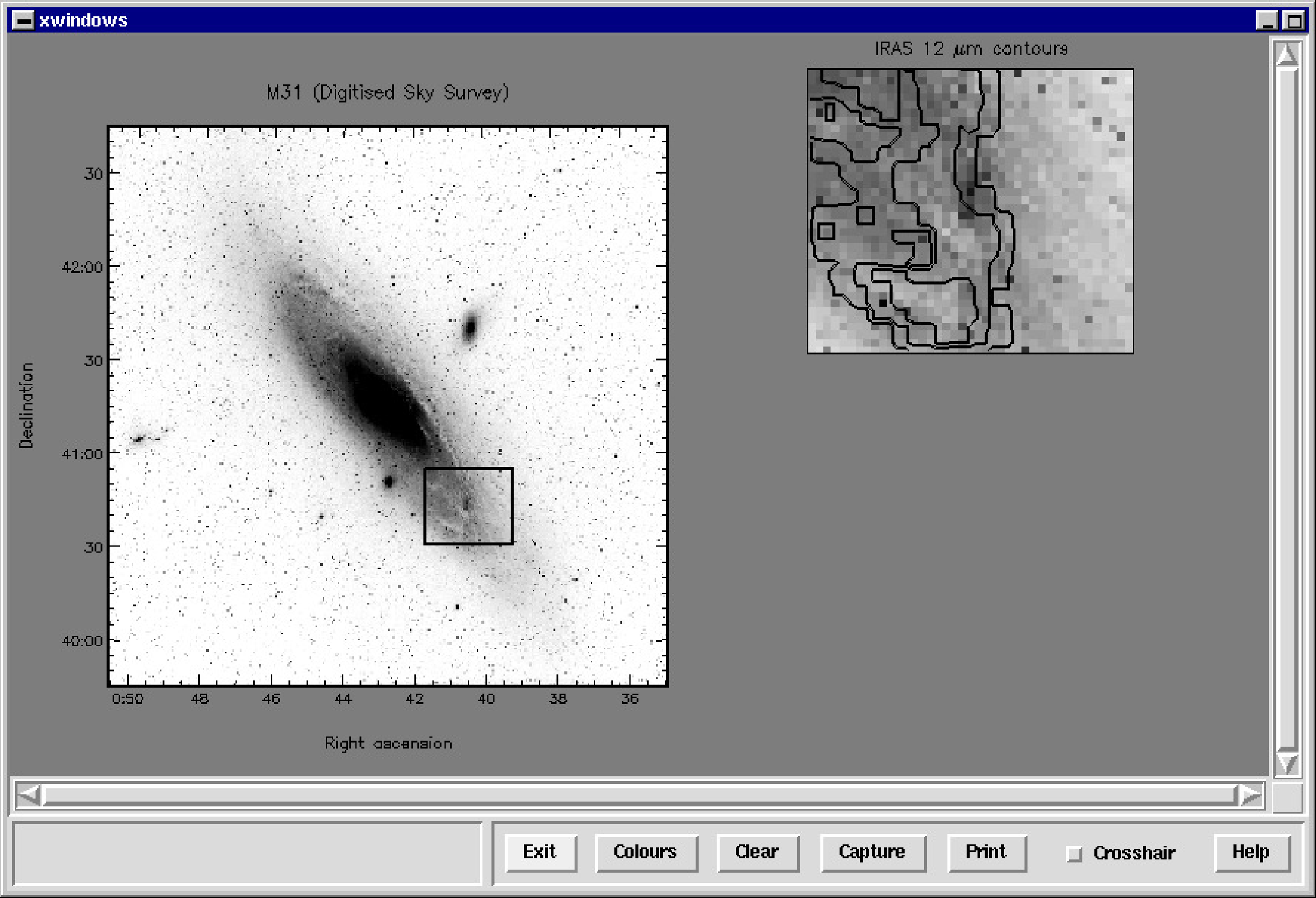
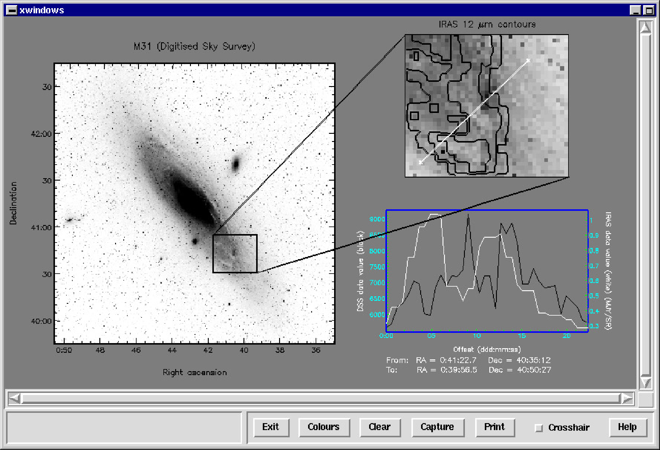
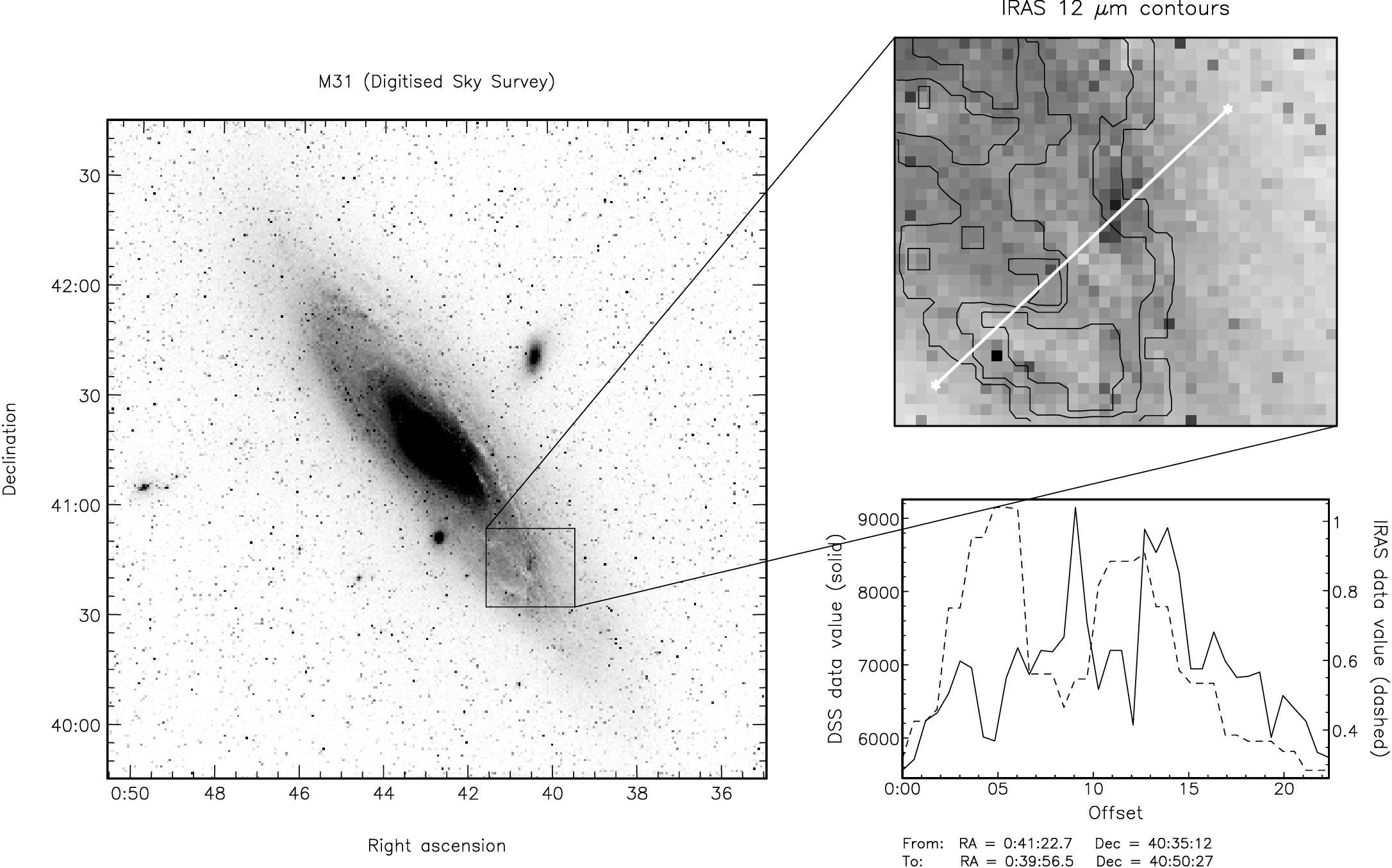
Remember the IRAS image of M31 we started with? We’ll now overlay contours of the IRAS image on top of the magnified section of the visual image we have just displayed. Don’t forget, these two images have not been aligned—for instance, north is up in the visual image, but down in the IRAS image. However, both images have information within the WCS component describing the relationship between pixel co-ordinates and RA/DEC. This WCS information was stored with the DATA picture created by DISPLAY above, and so can be used by the CONTOUR application in order to draw the IRAS contours in alignment with the displayed visual image.15 In addition, we also use CURSOR to mark a position with a text string giving a title for the contour plot:
The X-window should now look like Figure 5.
The most important parameter in the above invocation of CONTOUR is the NOCLEAR keyword (equivalent to CLEAR=NO). This tells CONTOUR not to clear the graphics device before drawing the contours. Instead, CONTOUR looks for an existing DATA picture contained within the current picture. If one is found, then CONTOUR attempts to align the contours using the WCS information stored with the existing DATA picture. In our case, the current picture is still the top-right FRAME picture created by PICDEF, and so the contours are aligned using the WCS information stored with the DATA picture contained within this FRAME picture (i.e. the magnified image section). CONTOUR tells us that this alignment occurred within the ‘SKY Domain’—if either of the two NDFs had not contained a calibration in a suitable celestial co-ordinate system, then alignment on the sky could not have been performed. In this case, CONTOUR would have aligned the contours in the ‘PIXEL Domain’ (i.e. in pixel co-ordinates).
Since we produced no annotated axes, a title string was added using the text drawing
abilities of CURSOR. The pointer was positioned above the contour plot, and the left
button clicked. The specified text string was drawn centred at this cursor position.
Note, the string \gm is a ‘PGPLOT escape sequence’ that represents the Greek letter mu
("μ").
See the PGPLOT manual for a detailed description of the available escape sequences.
Let’s say we wanted to compare the data values in the visual and IRAS images along a given line through the magnified sub-section. To do this, we first use the application PROFILE to create a pair of one-dimensional NDFs containing the data values along the line in each of the two images. We then display these one-dimensional NDFs using application LINPLOT. First we choose the line along which the profiles are to be taken, using CURSOR (again!):
The pointer is positioned at the two ends of the required profile, and the left button clicked at
each position. The supplied positions are marked by two markers of PGPLOT type 3 (small
crosses), and a white line is drawn between them (forming a ‘chain’). The selected positions
are written to an output catalogue stored in file zz.FIT. We now sample the data in the
two images along this profile to create a pair of one-dimensional NDFs (m31_prof and
iras_prof):
We want to draw the two line profiles in a new plot in the clear area at the bottom right of the X-window. We therefore need to create a new FRAME picture. This time we use PICDEF in ‘XY mode’, in which the bounds of the new FRAME picture are given explicitly using parameters UBOUND and LBOUND (we could have used cursor mode again; we use XY mode just to explore the different possibilities):
The bounds are supplied in the BASEPIC Frame (the bounds reported by the application are the bounds of the entire BASE picture). The new FRAME picture is, as usual, made the current picture by PICDEF and so any subsequent graphics applications will draw in the new FRAME picture.
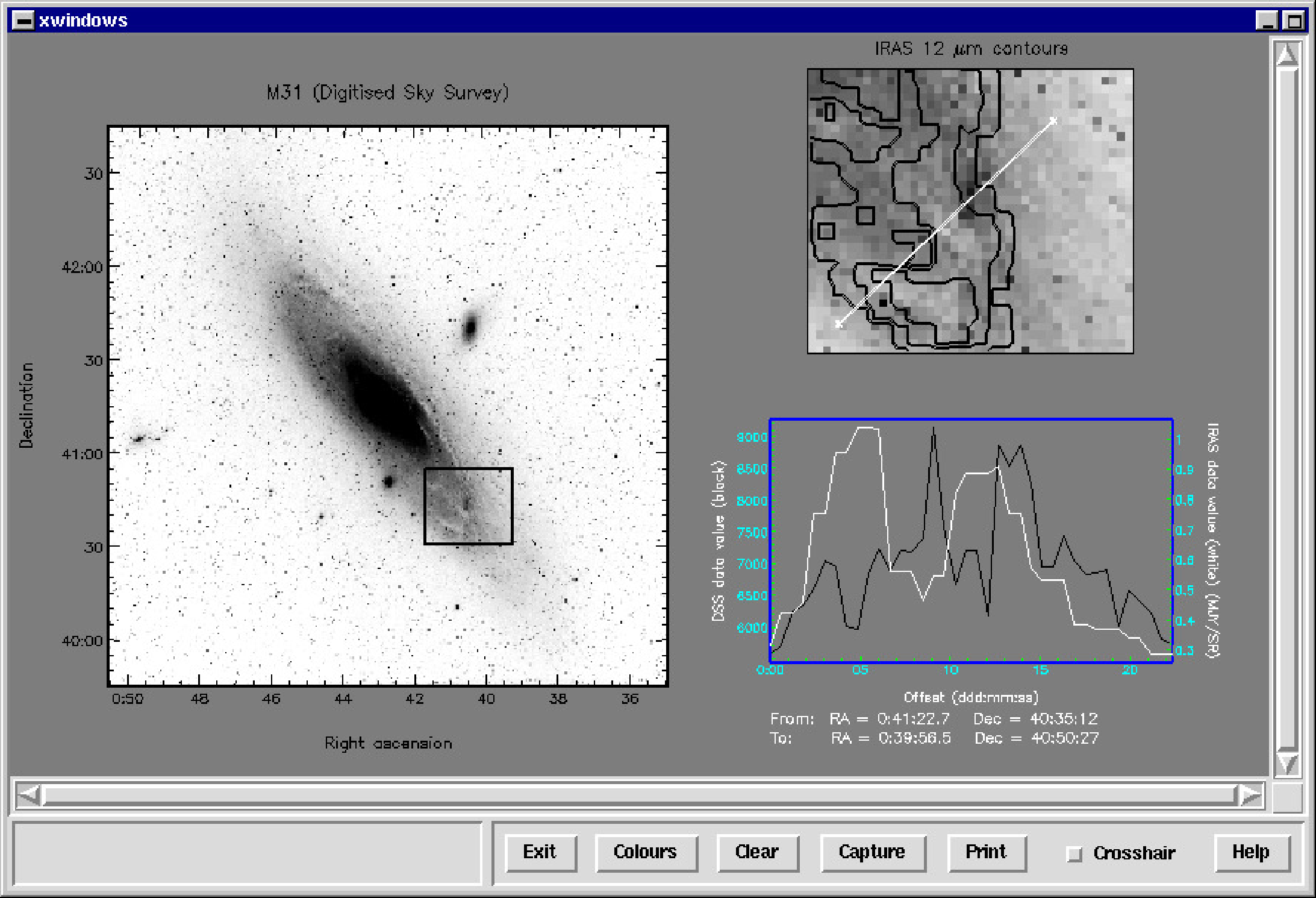
We now draw the first of the two line profiles:
The X-window should now look like Figure 6. The plotting attributes specified by the STYLE parameter do the following; tickall=0 stops tick marks from being drawn on the un-labelled edges (i.e. the top and right edges); colour(curve)=black specifies that the data curve is to be drawn in black; drawtitle=0 prevents a title being drawn at the top of the plot; label(2)=DSS data value (black) specifies the textual label for the left hand edge.
We now draw the second line plot over the top of the first line plot:
Again, the NOCLEAR keyword prevents LINPLOT from clearing the graphics device before drawing the new line plot. Instead, the new line plot is drawn within the same axes as any existing line plot within the current picture. By default, the new line plot would adopt the bounds of the two existing axes. This would be inappropriate in this case since the two images have very different data scales. To prevent this, we specify the NOALIGN keyword, which causes the default bounds for the new axes to be determined from the supplied data instead of the existing line plot. The STYLE parameter is similar to the previous line plot except that the data values are annotated on the right hand edge (edge(2)=r), the data curve is drawn in white, and data label is different.
The X-window should now look like Figure 7.
As a final touch, we will add two ‘warp’ lines to the display joining the corners of the box marking the enlarged image area to the corresponding corners on the enlarged image. CURSOR can be used to draw these lines, but we need to take a little care. Normally, graphics produced by CURSOR will be clipped at the edge of the picture in which the supplied positions fall. In our case, the required lines start in one picture (the main image display DATA picture), but end in another (the magnified image DATA picture). To avoid the lines being clipped when they leave the main image DATA picture, we first ensure that the current picture is the BASE picture (i.e. the whole screen), and we tell CURSOR to report positions within the current picture. Normally, CURSOR reports each position within the most recent picture under the cursor, but setting parameter MODE=CURRENT when running CURSOR means that the reported positions always refer to the co-ordinate system of the current picture. So, first make the BASE picture the current picture. This is done using PICLIST, remembering that the BASE picture is always picture number 1:
We now run CURSOR to draw the first warp line:
Position the pointer over the top left corner of the black box marking the selected image section in the main image display, and click the left button. Then position the pointer over the top left corner of the border surrounding the enlarged image display, and click again. A line is drawn between these two points.
We now run CURSOR again to draw the second warp line:
Point and click over the bottom right corners of the two boxes this time. The final X-window should look now look like Figure 8.
Various other facilities related to the graphics database exist as well as those described in the previous section. This section gives a brief description of a few more:
will give the label FRED to the current picture. This picture could be made current again at a later time by re-selecting it using PICSEL:
Any label associated with a picture is displayed in the list produced by PICLIST.
The bottom-left picture would be labelled SPEC1 and the rest are numbered in sequence from
left to right to SPEC12—the top-right picture. You’d call PICSEL to select each picture in turn via
a while loop in a C-shell script (see Section 19.1). Since this is a common operation a shorthand
command, PICGRID, is available. For instance:
is equivalent to the previous example, except that the pictures are labelled 1 to 12.
DATA, because of the
rule that applications must not change the current picture. Another way to select a new current
picture is via the command PICCUR. It displays a cursor. Move the cursor to lie on top of the
picture you require and select a point following the instructions (usually by pressing
the left-button of the mouse), then exit (normally by hitting the right-hand mouse
button). Generally, this will be fine, but you can have cases where one plot is still
visible through a transparent plot drawn subsequently. If the later picture extends
entirely over the image you require, PICCUR will not let you access it. The moral is “be
careful when arranging your pictures”. A picture may only be partially obscured, so
by moving the cursor around and hitting the left-hand button you can often find
a portion that is topmost. PICCUR reports the name, comment and the label (if it
there is one) of the picture in which the cursor is located to assist you. It is usually
quite obvious where pictures begin and end, so in practice it is easier than described
here.
Each picture in the graphics database has associated with it several co-ordinate Frames. Some of these describe positions within the displayed data array, and others describe the corresponding positions on the graphics device. Each Frame is referred to by a Domain name (see Section 12.2 for more information about co-ordinate Frames and Domains).
The following Domains may be used to specify positions within any picture:
DATA pictures have additional co-ordinate Frames inherited from the WCS information (see Section 12) associated with the displayed data. The details of the available Frames will depend on the application that created the picture and the nature of the data. For instance, if an image is displayed in which the current Frame is a SKY Frame (calibrated in RA/DEC for instance), then the Domains GRID, PIXEL, AXIS and SKY will also be available.
Pictures created by older applications that do not yet support WCS information will not have all of these Frames. They will still have GRAPHICS, BASEPIC, NDC and CURPIC Frames, but the only additional Frames will be:
The interpretation of both these Frames will depend on the application that created the picture, and should be described in the associated documentation. Note, the AGI_DATA Frame may not always be present. This again depends on the application.
The location of the graphics database file can be controlled by setting the
environment variable AGI_USER to the desired location. If AGI_USER is undefined,
the database file is placed in your home directory. Thus by default the file is
$HOME/agi_<node>.sdf,
where you substitute your computer’s node name for
<node>,
e.g. /home/dro/agi_rlsaxp.sdf. A new database is created when you run a graphics application if
none exists. AGI will purge the database for a device if the graph window has changed size, or if you
switch between portrait and landscape formats for a printer device.
The contents of the graphics database are ephemeral. Therefore you should regularly purge the database entries with GDCLEAR or delete the database file.
If a graphics application is aborted abnormally (for instance by pressing CTRL/C), the graphics
database may be corrupted, potentially resulting in various forms of peculiar behaviour when
subsequent graphics applications are run. If you get ‘strange’ behaviour when running a
graphics application, deleting the graphics database file and starting again will often cure the
problem.
Having produced a pretty picture in an X-window, how do we get it on to a piece of paper? There
are basically two ways. The simplest way is to do a screen-shot (i.e. copy the pixel values
from the X-window into a PNG file, or some other suitable graphics format), and then
print the file on a suitable printer. There are many ways to do this, depending on your
operating system (GIMP, ImageMagick, ksnapshot, print screen, etc). The figures in this
chapter were created using this method. It’s easy—but the results only have the resolution of
your X screen (typically 72 dots per inch) which is usually not good enough for general
publication.
The second method is more involved, but retains the full resolution of your printer (typically 600 dots per inch or more), producing far superior results. It involves running all the Kappaapplications again, but using a suitable encapsulated PostScript graphics device instead of the X-windows device used earlier in this chapter. Each application will then write its graphical output to one or more disk files. If you elect to use one of the “accumulating” PostScript devices (as indicated in the device description displayed by GDNAMES), then the PostScript output from each application will be merged automatically into a single file. If you use one of the other PostScript devices, each application will produce a separate output file, all of which must be combined using PSMERGE to create a single PostScript file containing the entire plot, which can be printed or included in another document.
We will look at these method in more detail in the rest of this section.
If you want to combine the results of several applications into a single plot, you need to specify an encapsulated PostScript device. These differ from normal PostScript files in that they contain information which allows them to be included within other PostScript files. The GDNAMES command displays a list of all the available graphics devices, together with a brief description of each. This should enable you to select an appropriate device name.16 There may be various encapsulated PostScript devices available. For instance, you can choose between colour or monochrome devices, and between portrait or landscape devices. The choice of colour or monochrome obviously depends on the printer you will use. The choice of landscape or portrait depends on the shape of the total plot you are producing—for tall narrow plots choose portrait, for short wide plots choose landscape.17
Creating composite graphical output will be easier if you choose one the devices that are described as “accumulating”, as this will avoid the need for you to merge separate PostScript files yourself.
For instance, if you want all applications to write graphical output to a single colour landscape encapsulated PostScript file set the graphics device as follows:
Having selected a suitable encapsulated PostScript graphics device, each Kappa application will
either modify an existing graphics file, or produce an new output file in your current directory
containing PostScript commands, depending on whether you choose an accumulating device or not.
These files can be examined without needing to be printed by using OKULAR, EVINCE, ghostview, etc.
By default, the output file will be called pgplot.ps.
Note, if you choose not to use an accumulating device, subsequent graphics commands
will overwrite any file created by earlier graphics commands. For this reason you should
rename the output file after running each graphics command. An alternative approach is
to assign a unique value to the DEVICE parameter for each graphics command (rather
than just allowing it to default to the value of the global parameter set using GDSET). For
instance, DEVICE="epsf_l;contour.ps" would cause the command to write its output to
file contour.ps.
This section is only relevant if you are using a non-accumulating device.
Once all applications have been run, you will have a potentially long list of PostScript files in your current directory (unless you use an accumulating device, in which case you will have only one). These need to be stacked together to produce a single PostScript file which can either be printed or included in a document. To do this, we use PSMERGE as follows18:
This stacks the three specified PostScript files into a single file called total.ps. This will be a normal
(i.e. not encapsulated) PostScript file, so you can print it, but it will be difficult to include it in a
document. If you include the -e option when running PSMERGE, then an encapsulated PostScript file
is created instead:
The output file can be included in other documents but often causes problem when being printed.
Note, the order in which you supply the input files is important because later files are pasted ‘on top of’ earlier files, and so can potentially obscure them. In general, you need to list the input files in the order in which they were created.
PSMERGE has other facilities which allow you to scale, shift and rotate individual input files before including them in the output. See SUN/164 for details.
The main difference between producing X-window output and PostScript output is that there is no
cursor available when using PostScript. This means, for instance, that you cannot use PICDEF in
cursor mode, and you cannot use CURSOR at all! We made use of both these facilities when we
produced Figure 8. Pictures must be defined using PICDEF in XY mode, or one of the other
positional mode (CC, BL, etc.). Annotation such as produced by CURSOR can be created using
LISTMAKE and LISTSHOW. You specify the reference positions for the annotation in any
suitable co-ordinate Frame using LISTMAKE. This creates a positions list file containing
these positions, together with associated WCS information. You then supply this file to
LISTSHOW which marks the positions on the graphics device in any of the ways provided by
CURSOR.
It can often be advantageous to design your final plot using an X-windows graphics device. This provides more versatility in the form of a graphics cursor and dynamic lookup table, and also allows you to see the plot more easily. Once the plot looks right in the X-window, you can then run the drawing commands again specifying a suitable PostScript device instead.
If you choose to do this, it can be a big help to ensure that the X-window you are using has the same shape as your selected PostScript device. This prevents you accidentally drawing things within regions of the X-window that are not available in PostScript. To find the require aspect ratio, do:
This clears the PostScript device, and then displays the bounds of the BASE picture (all the other pictures were erased by GDCLEAR). The results will look something like this:
This tells you that the aspect ratio (the ratio of the width to the height) of the PostScript device is 1.455. You should now make an X-window with this aspect ratio:
The xdestroy command deletes any existing X-window, and the xmake command creates a new one
with a height of 500 pixels and a width of 730 pixels, giving the required aspect ratio. Of course, you
could produce a larger or smaller X-window so long as the ratio of width to height is close to
1.455.
Another tip to ease prototyping on an X-window—when you run CURSOR, always store the selected positions in an output positions list, using Parameter OUTCAT. When you come to produce the PostScript files, you can then supply these positions lists as inputs to LISTSHOW, in order to mimic the annotation produced by CURSOR when you were prototyping.
As an illustrated example, this section describes how to produce a PostScript file containing a plot similar to that in Figure 8. For clarity (at the time), the earlier sections of this chapter did not adhere to either of the tips given above when prototyping in an X-window; that is, we did not choose the shape of the X-window to match our PostScript device, and we did not save the output from each run of CURSOR in a positions list file. For this reason, the steps taken here are a little more complicated than they need to be, and do not mimic exactly the steps taken while prototyping.
First, select and clear the graphics device. We choose a accumulating, monochrome, portrait, encapsulated PostScript device:
Since we are using an accumulating PostScript device, we have chosen to use OKULAR above to
display the contents of pgplot.ps. We have just run GDCLEAR, and so this will produce a blank
display. Note that we have put OKULAR into the background by appending & to the end of the
command line. This means that OKULAR will continue to run throughtout the following example. As
each subsequent graphics application modifies the contents of pgplot.ps, the resulting
composite plot will be displayed immediately within the OKULAR window, allowing you
to review progress. Other modern document viewers such as EVINCE work in the same
way.
In order to produce higher quality axis annotations, we now tell PGPLOT to use embedded PostScript fonts rather than it’s own internal lower-quality fonts. Specifically, we use a Times New Roman font:
We could instead have set PGPLOT_PS_FONT to “Helvetica”, “Courier”, “NewCentury” or “Zapf”, to
use other fonts.
We will sometimes need to specify positions within the BASE picture. To do this we can either use the GRAPHICS, the BASEPIC or the NDC Frame, all of which span the entire graphics device. GRAPHICS is an absolute co-ordinate system giving millimetres from the bottom left corner of the graphics device, and BASEPIC is a normalised co-ordinate system in which both axes have the same scale and the shorter dimension of the graphics device has length 1.019. The BASEPIC Frame is usually easier to work with since it does not depend on the size of the paper. To determine the bounds of the available plotting space in the BASEPIC Frame, use GDSTATE, having first ensured that the BASE picture is the current picture (this will be the case at the moment since we have just cleared the database using GDCLEAR):
The choice of a portrait PostScript device may have surprised you, given that Figure 8 seems more naturally to fit into a landscape page. Portrait mode was chosen so that the final plot appears up-right when included in a document. If landscape mode had been chosen, the final plot would have been rotated by 90° when included in a latex document such as this one, requiring the page to be viewed on its side. However, if we use the entire portrait page, we will have too much vertical space between the components of the plot. To avoid this we only use the bottom third (roughly) of the page—that is, we pretend that the top of our ‘page’ is at 0.6 instead of 1.454659.
We first create a FRAME picture at the left hand side of the page covering the full height of our reduced ‘page’ and 0.6 of the width. We specify the upper and lower bounds of the picture within the BASEPIC Frame, using the limits found above, giving the FRAME picture the label ‘main’ so that we can easily re-select the picture later. We then display the optical image within it, including annotated axes:
Note, we are using a monochrome PostScript device, and so the colour of all annotation produced by DISPLAY was set to black using the STYLE parameter. This is done for all applications that produce graphical output. We also request text 0.6 of the default size. We specified the MARGIN parameter when running DISPLAY in order to reduce the margin on the right hand side of the image. By default, DISPLAY leaves a margin equal to 0.2 of the width of the DATA picture. We reduced this to 0.02 to make more room for the other components of the plot (the first value supplied for MARGIN is the bottom margin and is left at 0.2).
We now draw a box over this image to mark the ‘selected region’ indicated in Figure 3. In this particular case, we use LISTMAKE to create a positions list holding the RA and DEC at the two opposite corners of the box. Alternatively, we could have saved the output from CURSOR while prototyping, using the OUTCAT parameter. In either case, we use LISTSHOW to draw the box:
Note, the PostScript output generated by LISTSHOW is merged automatically into the pgplot.ps file
created by the previous graphics applications. If we had chosen not to use an accumulating device, we
would need to rename the new pgplot.ps file created by each graphics application, and then merge
them all together at the end using PSMERGE.
Specifying ndf=m31 resulted in LISTMAKE interpreting the supplied positions as positions within the
current co-ordinate Frame of the NDF m31. It also results in all the WCS information being copied
from the NDF into the output positions list.
We now create a Frame in the top-right corner of the reduced ‘page’ in which a magnified image of the selected region will be displayed. The picture occupies the remainder of the width left over by the main image (0.4 of the total width) and half the height.:
We now display the selected image section within the FRAME picture just created, and overlay
contours from iras.sdf. We draw the border with twice the default width:
What are those two extra commands in the middle? Well, we will need to be able to re-select the DATA
picture holding the image when we come to draw the warp-lines. To do this we need to label
the picture now. For this reason, we use PICDATA to select the DATA picture created by
DISPLAY as the current picture, and then use PICLABEL to give the label "mag" to the
picture.
We now display a title above this DATA picture. The string is centred horizontally within the enclosing FRAME picture (i.e. half way between 0.6 and 1.0), and drawn so that its bottom edge is placed at the top of the Frame:
LISTMAKE is used to store the position in a positions list, and then LISTSHOW is used
to draw the title. Again, we could have saved the output from CURSOR in a positions
list while prototyping, instead of using LISTMAKE to create the positions list. The JUST
parameter is set to bc so that the title string is displayed with its bottom centre at the supplied
position.
We now draw the line marking the path of the profiles that will be displayed later. We draw them in white so that they show up against the predominantly dark background of the image:
The line is drawn with three times the default width. We now create the profiles as before:
We now create a FRAME picture occupying the remaining area at the bottom right corner of the page, and display the two profiles in it. We use line style to differentiate the two curves, instead of colour as we did when prototyping:
The appearances of the two plots are controlled by the two plotting styles contained in the text files
style1 and style2. style1 contains the following attribute settings:
The file style2 contains the following attribute settings:
Now comes the complicated bit—the warp lines! The problem is that we used the cursor to define the start and end of these lines when prototyping. This was good enough for an X-window that has relatively low resolution, but will not do for PostScript. We cannot place the cursor accurately enough to ensure that there is no visible gap between the end of the line and the corresponding box corner when using PostScript, so we cannot use the positions found while prototyping. The only way to ensure that the lines join up properly with the box corners is to use the co-ordinates of the box corners to define the lines. First, we need to transform the box corners into the BASEPIC Frame since both ends of each line must be given within the same co-ordinate Frame.
We start with the ‘selection box’ drawn over the main image. The corners of this box are currently
stored in the boxpos positions list. This file contains the RA and DEC at the corners of the box,
together with WCS information copied from the NDF m31. But this does not include the
BASEPIC, NDC or CURPIC Frame, which are only available within the WCS information
stored with graphics database pictures. In order to find the BASEPIC co-ordinates at the
corners of the box, we need to align the RA/DEC values in the positions list with the WCS
information stored with the first DATA picture we created (the main image), and then
display the corresponding BASEPIC co-ordinates. LISTSHOW can do this, but we need to
change the current picture first. At the moment, the current picture is the FRAME containing
the line plots. If we did not change the current picture LISTSHOW would assume that
the supplied RA/DEC values refer to the line plots (not to the main image), and would
consequently give the wrong BASEPIC co-ordinates. We use PICSEL to select the FRAME
picture containing the main image (so that it becomes the current picture), and then run
LISTSHOW:
The parameter assignment PLOT=BLANK tells LISTSHOW to search the graphics database for a picture
with which the positions in boxpos can be aligned, but without marking the positions in any way on
the screen. Doing this means that the co-ordinate Frames stored with the picture are available when
specifying a value for Parameter FRAME. This is necessary because the BASEPIC Frame is
only available within graphics data base pictures since it describes positions on a graphics
device.
We now find the BASEPIC co-ordinates at the corners of the magnified image. The most simple way of doing this is to use the same RA/DEC positions. The problem with this approach is that the bounds of the magnified image were rounded to a whole number of pixels and so may not correspond exactly to the RA an DEC at the corners of the selection box. A more accurate method is to use the pixel indices at the corners of the image section to define the box corners. We first need to create a positions list holding the pixel co-ordinate bounds of the image section, remembering to reduce the lower pixel index bounds by 1.0 in order to convert the integer pixel indices into floatingpoint pixel co-ordinates (see Section 12.1 for more information about pixel co-ordinates and indices):
We now need to use LISTSHOW to get the corresponding BASEPIC co-ordinates, aligning the above PIXEL co-ordinates with the DATA picture holding the magnified image section. Another slight complication arises here since the required DATA picture is obscured by the DATA picture holding the IRAS contours. Pixel co-ordinates in the IRAS image are totally different to those in the grey-scale image, and so we need to make sure that LISTSHOW is using the correct DATA picture. However, we labelled the required DATA picture when it was created and so we can just use PICSEL to re-select it:
We now create a positions list containing the BASEPIC co-ordinates at the ends of the upper warp line, and draw it. By default, LISTSHOW draws within the most recent DATA picture contained within the current picture. Since the line is not contained within a single DATA picture, we need to tell LISTSHOW to draw within the BASE picture. This is done by setting Parameter NAME to BASE (we also revert to drawing in black):
The last drawing we need to do is to create the second warp line in the same way:
That’s it. The final output is left in file pgplot.ps and should be visible in the OKULAR window. It
should look like Figure 9. However, if we had chosen not to use an accumulating PostScript device,
we would now be left with lots of PostScript files—one from each graphics application—that now
need to be stacked together to produce the final encapsulated PostScript file:
Note, here we assume that each pgplot.ps file has been renamed to one of the above names
immediately after it has been created, in order to avoid it being over-written by the next graphical
application.
10“AGI” is the name of the subroutine library that provides access to the graphics database. AGI stands for “Applications Graphics Interface”, and is documented in SUN/48.
11This rule does not apply to applications that manage the database itself rather than producing graphical output. Thus,
for instance, it is legal for PICLIST to change the current picture if you request such a change. Also, an uncontrolled exit
from an application, e.g. CTRL/C may leave the database in an abnormal state.
12The current co-ordinate Frame in the image being used is RA/DEC and so the axis will be annotated in RA and DEC.
13Pixel co-ordinates are fractional, where-as pixel indices are integer. The pixel with indices (1,1) covers a range of pixel co-ordinates between 0.0 and 1.0 on each axis, with its centre at pixel co-ordinates (0.5,0.5).
14Note, by default, the FRAME picture created by PICDEF is not constrained to be within the current picture, it can be anywhere within the BASE picture.
15The accuracy of this alignment will depend on the accuracy of the astrometry information supplied with the image.
16Most encapsulated PostScript devices start with the string "epsf" or "aps".
17The choice or portrait or landscape may also affect the orientation of the plot when the resulting PostScript file is included in a document.
18You can include all the PostScript files, including any that do not contain any actual drawing commands.
19NDC is like BASEPIC but the top-right corner of the device has NDC co-ordinates (1, 1).