15 Masking, Bad Values, and Quality
Masking is the process by which you can exclude portions of your data from data processing or
analysis. Suppose that you are doing surface photometry of a bright galaxy, part of the data
reduction is to measure the background contribution around the galaxy and to subtract it.
You usually want to avoid inclusion of light from the galaxy in your estimation of the
background. A convenient method for doing this is to mask the galaxy during the background
fitting.
There are two techniques used for masking. One employs special bad values (also known
as magic or invalid values). These appear within the data or variance arrays in place of
the actual values, and indicate that the pixel is to be ignored or is undefined. They are
destructive
and so some people don’t like them, but you can always mask your data into a new, temporary NDF.
With a little care, bad values are quite effective and they are used throughout Kappa. By its nature, a
bad value can only indicate a logical, two-state condition about a data element—it is either good or
bad—and so this technique is sometimes called flagging.
In contrast, the second technique, uses a quality array. This permits many more attributes or qualities
of the data to be associated with each pixel. In the current implementation there may be up to 255
integer values, or 8 single-bit logical flags. Thus quality can be regarded as offering 8 logical masks
extending over the data or variance arrays, and can signify the presence or absence of a particular
property if the bit has value 1 or 0 respectively. An application of quality to satellite data might
include the detector used to measure the value, some indicator of the time each pixel was
observed, was the observation made within the Earth’s radiation belts, and whether or not the
pixel contains a reseau mark. By selecting only those data with the appropriate quality
values, you process only the data with the desired properties. This can be very powerful.
However, it does have the drawback of having to store at least an extra byte per pixel in your
NDF.
The two methods are not mutually exclusive; the NDF permits their simultaneous use in a
dataset.
Now we’ll look at both of these techniques in detail and demonstrating the relevant Kappa tasks.
15.1 Bad-pixel Masking
Bad pixels are flagged with the Starlink standard values (see Section 5 of SUN/39), which for _REAL
is the most-negative value possible.
In addition to tasks that routinely create bad values in the output value is undefined, Kappa offers
many applications for flagging pixels with certain properties or locations.
15.1.1 Doing it the ARD Way
To mask a region or a series of regions within an NDF, you can create an ASCII Region Definition
(ARD) text file. ARD has a powerful syntax for combining regions and supplying WCS information,
described fully in SUN/183. An ARD file comprises keywords that define a region, such as RECT to
specify a rectangular box; operators that enable regions to be combined, for instance .AND. that will
form the intersection of two regions; and statements to define the world co-ordinate system and
dimensionality. For further details see the three sections called Regions, Operators, and Statements in
SUN/183.
Here is an example of the creation of an ARD file.
% cat myard.ard
COFRAME(PIXEL)
PIXEL( 23.5, -17.2 )
ELLIPSE( 75.2, 296.6, 33, 16, 78 )
POLYGON( 109.5, 114.5, 122.5, 131.5, 199.5, 124.5 )
CIRCLE( 10, 10, 40 ) .AND. .NOT. CIRCLE( 10, 10, 30 )
COFRAME(SKY,SYSTEM=FK5,EQUINOX=2000)
CIRCLE( 10:09:12.2, -45:12:13, ::40 )
CTRL/D
The COFRAME statements indicate the co-ordinate system in which subsequent positions are
supplied. Its first argument is the domain. Here the first COFRAME(PIXEL) refers to pixel
co-ordinates. Note that these are not the same as pixel indices, as they are displaced by
0.5 with
respect to pixel indices. The second COFRAME selects a SKY domain using the FK5 system, so that
regular equatorial co-ordinates may be supplied as arguments to subsequent keywords. Other
possible values for System include ECLIPTIC and GALACTIC. If no COFRAME or WCS
statement is present, the default co-ordinate system is pixel co-ordinates transformed by
any COEFFS, OFFSET, TWIST, STRETCH, SCALE statements. Note that the ARDMASK
application, used to mask data with an ARD file, has a DEFPIX parameter where you can choose
whether the default co-ordinates are pixel or those of the current WCS Frame. if there is no
COFRAME or WCS statement in your ARD file. Still you are recommended to supply a
COFRAME or WCS statement in your ARD files to avoid accidentally selecting the wrong
regions.
In this example, the regions are: the single pixel at co-ordinates (23.5, -17.2); an ellipse
centred at (75.2, 296.6) with semi-major axis of 33 pixels and semi-minor axis of 16 pixels, at
orientation 78° clockwise from the x axis; a triangle with vertices at pixel indices (110, 115),
(123, 132), (200, 125); an annulus centred on pixel co-ordinates (10.0, 10.0) between radius
30 and 40 pixels; and a circle centred on RA 10:09:12.2, and DEC -45:12:13 of radius 40
arcseconds.
Operators combine regions using a Fortran-like logical expression, where each keyword acts like a
logical operand acted upon by the adjoinning operators. Statements are ignored in such logical
expressions. There is an implicit .OR. operator for every keyword on a new line. Thus pixels that lie in
any of the above regions (the union) are selected.
Where a keyword (such as CIRCLE, RECT, POLYGON) defines an area or volume a pixel is deemed to
be part of that region if its centre lies on or within the boundary of the region. For regions of zero
volume (such as keywords PIXEL, LINE, COLUMN), the pixel is regarded as part of the region when
the locus of the region passes through that pixel. So for example, a PIXEL region will be the pixel
emcompassing the supplied co-ordinates; and for a LINE, the selected pixels are all that intersect with
the line’s locus.
Here are some more examples of ARD files.
COFRAME(GRID)
ROTBOX( 12, 15, 20, 10, 36.3 ) .AND. .NOT. ( COLUMN( 13 ) .OR. ROW( 8 ) )
Now the co-ordinates are Grid co-ordinates. This selects all the pixels with a rotated box except those
in thirteenth column or eighth row. Note the use of parentheses to adjust or clarify the precedence.
The box is centred on grid pixel (12, 15) has sides of length 20 and 10 pixels. The first side of the
box—the one with length 20—is at an angle of 36.3° measured anticlockwise from the X axis.
DIMENSION(3)
CIRCLE( 10.3, 21.6, 32.9, 10.4 )
LINE( 1.1, 2.2, 3.3, 4.4, 5.5, 6.6 )
This defines a sphere centred at pixel co-ordinates (10.3, 21.6, 32.9) with radius 10.4 pixels, and a line
from (1.1, 2.2, 3.3) to (4.4, 5.5, 6.6).
CIRCLE( 10.3, 21.6, 32.9, 10.4 )
This defines a sphere centred at pixel co-ordinates (10.3, 21.6, 32.9) with radius 10.4 pixels.
.NOT. ELLIPSE( 75.2, 296.6, 33, 16, 78 )
This selects the whole array except for the ellipse defined as before. Something like this might be
useful for excluding a galaxy image before fitting to the background around the galaxy.
There are more details and further ARD facilities described in SUN/183. If you do not wish to
read SUN/183, you’ll be relieved to learn that there are shortcuts for two-dimensional
data…
The first is is provided by GAIA by its Image Analysis
Image
Regions… tool. Here you can select region types and interactively adjust the region locations and
shapes, and then record the selected regions in an ARD file. However, it does not provide the boolean
operators other than .OR. to combine a series of regions, or use co-ordinates other than
pixel.
Kappa offers its own interactive graphical tool for generating ARD files. To use ARDGEN you must
first display your data on a device with a cursor, such as an X-terminal. DISPLAY with a grey-scale
lookup table is probably best for doing that. The grey lets you see the coloured overlays clearly. The
following example assumes that the current co-ordinate Frame in the NDF is PIXEL (i.e. pixel
co-ordinates). Consequently all positions are shown below in pixel co-ordinates. If the
current co-ordinate Frame in the NDF was not PIXEL but (say) SKY, then ARDGEN would
produce positions in SKY co-ordinates. The ARD file generated by ARDGEN always contains
a description of the co-ordinate system in which positions are specified, allowing later
applications to interpret them correctly, and convert them (if necessary) into other co-ordinate
systems.
% ardgen demo.ard
Current picture has name: DATA, comment: KAPPA_DISPLAY.
SHAPE - Region shape /’CIRCLE’/ >
At this point you can select a shape. Enter ? to get the list. Once you’ve selected a shape you’ll receive
instructions.
SHAPE - Region shape /’COLUMN’/ > ellipse
Region type is "ELLIPSE". Identify the centre, then one end of the semi-major
axis, and finally one other point on the ellipse.
To select a position press the space bar or left mouse button
To exit press "." or the right mouse button
Once you have defined one ellipse, you can define another or exit to the OPTION prompt. In addition
to keyboard 1, pressing the right-hand mouse button has the same effect. Thus in the example, the
new shape is a rotated box.
Region completed. Identify another ’ELLIPSE’ region...
OPTION - Next operation to perform /’SHAPE’/ > shape
SHAPE - Region shape /’ELLIPSE’/ > rotbox
Region type is "ROTBOX". Identify the two end points of any edge and then give
a point on the opposite edge.
Region completed. Identify another ’ROTBOX’ region...
If you make a mistake, use the ‘Undo’ option. Alternatively, enter List at the OPTION prompt to see
a list of the regions. Note the ‘Region Index’ of the region(s) you wish to remove, and select the
Delete option. At the REGION prompt, give a list of the regions you want to remove. If you
change your mind, enter ! at the prompt for Parameter REGIONS, and no regions are
deleted.
Now suppose you want to combine or invert regions in some way, you supply Combine at the
OPTION prompt. So suppose we have created the following regions in $KAPPA_DIR/ccdframe.
Region Region Description
Index
1 - ELLIPSE( 174.1, 234.4, 82.2, -43.5, 65.64783 )
2 - ELLIPSE( 168.1, 209.1, 29.4, -19.7, 9.441798 )
3 - ELLIPSE( 42.2, 244.1, 13, -10.3, 111.8452 )
4 - ROTBOX( 40.5, 219.2, 63.8, 38.3, 37.24281 )
5 - RECT( 141.5, 1.4, 143.9, 358.8 )
6 - POLYGON( 229.8, 247.7,
233.4, 247.7,
233.4, 258.6,
231, 267,
229.8, 265.8,
228.6, 256.2 )
We want to form the region inside the first ellipse but not inside the second. This done in two stages.
First we invert the second ellipse, meaning that pixels are included if they are not inside this ellipse,
by combining with the NOT operator.
OPTION - Next operation to perform /’SHAPE’/ > comb
OPERATOR - How to combine the regions /’AND’/ > not
OPERANDS - Indices of regions to combine or invert /6/ > 2
This removes the original Region 2, decrements the region numbers of the other regions following 2
by one, so that Region 3 becomes 2, 4 becomes 3, and so on. A new Region 7 is the inverted ellipse.
The renumbering makes it worth listing the regions before combining regions. The second stage is to
combine it with Region 1, using the AND operator. This includes pixels if they are in both regions. In
this example, that means all the pixels outside the second ellipse but which lie within the
first.
OPTION - Next operation to perform /’SHAPE’/ > com
OPERATOR - How to combine the regions /’AND’/ >
OPERANDS - Indices of regions to combine or invert /[6,7]/ > 1,6
Here is another example of combination. This creates a region for pixels are included provided they
are in one of two regions, but not in both. Here we apply the .XOR. operator to the small ellipse and
the first rotated box.
OPTION - Next operation to perform /’SHAPE’/ > comb
OPERATOR - How to combine the regions /’AND’/ > xor
OPERANDS - Indices of regions to combine or invert /[4,5]/ > 1,2
Here is the final set of regions.
OPTION - Next operation to perform /’SHAPE’/ > list
Region Region Description
Index
1 - RECT( 141.5, 1.4, 143.9, 358.8 )
2 - POLYGON( 229.8, 247.7,
233.4, 247.7,
233.4, 258.6,
231, 267,
229.8, 265.8,
228.6, 256.2 )
3 - ( ELLIPSE( 174.1, 234.4, 82.2, -43.5, 65.64783 )
.AND.
( .NOT. ELLIPSE( 168.1, 209.1, 29.4, -19.7, 9.441798 ) ) )
4 - ( ELLIPSE( 42.2, 244.1, 13, -10.3, 111.8452 )
.XOR.
ROTBOX( 40.5, 219.2, 63.8, 38.3, 37.24281 ) )
Once you are done, enter "Exit" at the OPTION prompt, and the ARD file is created. "Quit" also
leaves the programme, but the ARD file is not made.
Having created the ARD file it is straightforward to generate a masked image with
ARDMASK:
% ardmask $KAPPA_DIR/ccdframec demo.ard ardccdmask
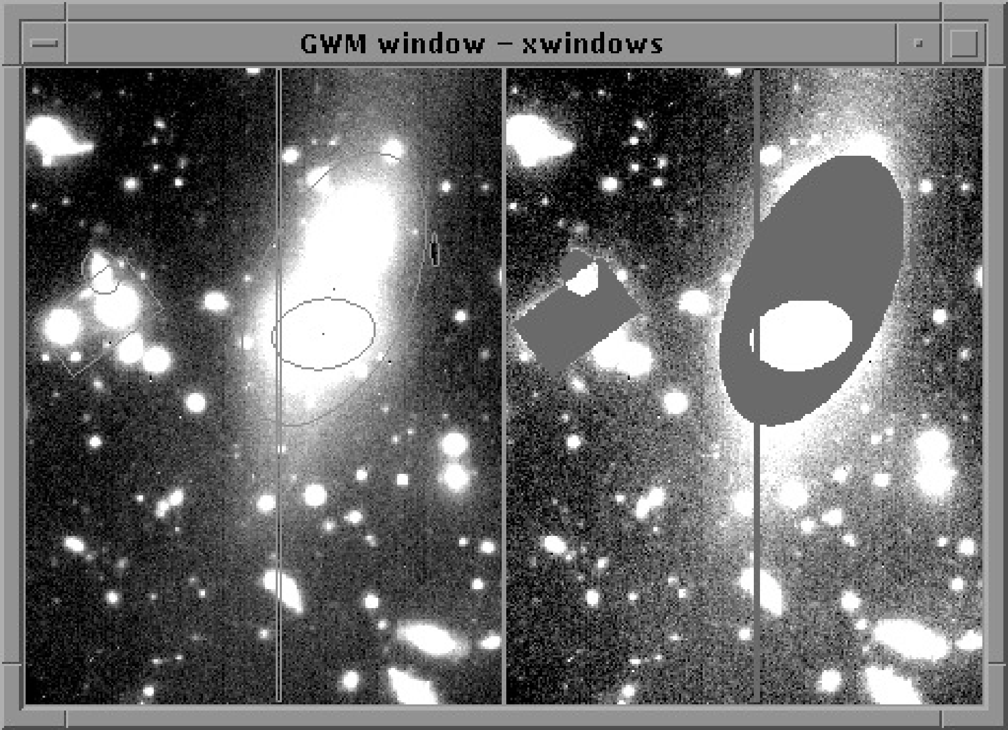
Figure 13 shows the image with the original regions outlined to the left. Note only the section
(:270, :360) is displayed. To see where you have masked, use DISPLAY, which lets you define a colour
for bad pixels using the BADCOL parameter.
% display ardccdmask badcol=red \\
To the right of Figure 13 is the final masked image.
15.1.2 SEGMENT and ZAPLIN
SEGMENT is ostensibly for copying polygonal regions from one NDF to another. You may also use
SEGMENT to copy bad pixels into the polygonal regions by giving the null value for one of the two
input NDFs. For instance,
% segment in1=! in2=$KAPPA_DIR/ccdframec out=ccdmask
NDF ccdmask will have bad values inside the polygons, whereas
% segment in2=! in1=$KAPPA_DIR/ccdframec out=ccdmask
the pixels exterior to the polygons are flagged. SEGMENT lets you define the polygon vertices
interactively, like in ARDGEN, but you can also use text files, or respond to prompting.
ZAPLIN also has an option to fill in rectangular areas when Parameter ZAPTYPE has value
Bad.
15.1.3 Special Filters for Inserting Bad Values
There are applications that mask pixels if their values meet certain criteria.
SETMAGIC flags those pixels with a nominated value. It is most useful during conversion of imported
data whose data system uses bad-pixel values different from Starlink’s.
FFCLEAN removes defects smaller than a nominated size from an image or vector NDF . It flags
those pixels that deviate from a smoothed version of the NDF by more than some number of standard
deviations from the local mean.
ERRCLIP flags pixels that have errors larger than some supplied limit or signal-to-noise ratios below a
threshold. The errors come from the VARIANCE component of the NDF. Thus you can exclude
unreliable data from analysis.
THRESH flags pixels that have data values within or outside some specified range.
15.2 Quality Masking
All the NDF tasks in Kappa use quality yet there is no obvious sign in individual applications how
particular values of quality are selected. What gives? The meanings attached to the quality bits will
inevitably be quite specific for specialist software packages, but Kappa tasks aim to be general
purpose. To circumvent this conflict there is an NDF component called the bad-bits mask that forms
part of the quality information. Like a QUALITY value, the bad-bits mask is an unsigned byte. Its
purpose is to convert the eight quality flags into a single logical value for each pixel, which can then
be processed just like a bad pixel.
When data are read from the NDF by mapping into memory, the quality of each pixel is combined
with the bad-bits mask; if a result of this quality masking is FALSE, that pixel is assigned the bad value
for processing. This does not change the original values stored in the NDF; it only affects the mapped
data.
So how do the quality and bad-bits mask combine to form a logical value? They form the bit-wise
‘AND’ and test it for equality for 0. None the wiser? Regard each bit in the bad-bits mask as a
switch to activate detection of the corresponding bit in a pixel’s quality. The switch is on if
it has value 1, and is off if it has value 0. Thus if the pixel is flagged only if one or more
of the eight bits has both quality and the corresponding bad-bit set to 1. Here are some
examples:
| QUALITY: | 10000001 | 10000001 |
| Bad-bits: | 01000100 | 01000101 |
| Bits on: | | ^ |
| Result: | TRUE | FALSE |
| |
The application SETBB allows you to modify the bad-bits mask in an NDF. It allows you to
specify the bit pattern in a number of ways including decimal and binary as illustrated
below.
% setbb RO950124 5
% setbb RO950124 b101
These both set the bad-bits mask to 00000101 for the NDF RO950124. SETBB also allows you to
combine an existing NDF bad-bits mask with another mask using the operators AND and OR. OR lets
you switch on additional bits without affecting those already on; AND lets you turn off selected bits
leaving the rest unchanged.
% setbb RO950124 b00010001 or
% setbb RO950124 b11101110 and
The first example sets bits 1 and 5 but leaves the other bits of the mask unaltered, whereas the second
switches off the same bits.
Now remembering which bit corresponds to which could be a strain on the memory. It would be
better if some meaning was attached to each bit through a name. There are four general tasks that
address this. SETQUAL sets quality values and names; SHOWQUAL lists the named qualities;
REMQUAL removes named qualities; and QUALTOBAD uses a logical expression containing the
named quality properties to create a copy of your NDF in which pixels satisfying the quality
expression are set bad. See Section 16 for more information about using these tasks. Once you have
defined quality names, you can set the bad-bits mask with SETBB to mask pixels with those named
quality attributes.
% setbb RO950124 spike
% setbb RO950124 ’"spike,back"’
The first example might set the bad-bits mask to exclude spike artefacts. The second could mask both
spikes and background pixels. Thus it might be used to select the spectral lines not affected by noise
spikes in a spectral cube. Other logical combinations are possible using the AND and OR
operators.
15.3 Removing bad pixels
Sometimes having bad pixels present in your data is a nuisance, say because some application outside
of Kappa does not recognise them, or you want to integrate the flux of a source. Kappa offers a
number of options for removing bad values. Which of these is appropriate depends on the reason why
you want to remove the bad pixels.
First you could replace the bad values with some other reasonable value, such as zero.
% nomagic old new 0 comp=all
Here dataset new is the same as dataset old except that any bad value in the data or variance array has
now become zero.
If you wanted some representative value used based upon neighbouring pixels, use the GLITCH
command.
% glitch old new mode=bad
This replaces the bad values in the data and variance arrays with the median of the eight
neighbouring pixels. This works fine for isolated bad pixels but not for large blocks. If your data are
generally flat, large areas can be replaced using the FILLBAD task.
The value of Parameter SIZE should be about half the diameter of the largest region of bad pixels.
Both the data array and variance arrays are filled.
You may replace individual pixels or rectangular sections using CHPIX.
% chpix old new
SECTION - Section to be set to a constant /’55,123’/ >
NEWVAL - New value for the section /’60’/ >
SECTION - Section to be set to a constant /’1:30,-10:24’/ >
NEWVAL - New value for the section /’-1’/ >
SECTION - Section to be set to a constant /’1:30,-10:24’/ > !
This replaces pixel (55, 123) with value 60, and the region from
(1, 10) to
(30, 24) with 1.
The final ! ends the loop of replacements. If you supply NEWVAL on the command line, only one
replacement occurs.
It is also possible to paste other datasets where your bad values lie with the PASTE and SEGMENT
tasks.
% paste old fudge"(10:20,29:30)" out=new
The dataset old is a copy of dataset new, except in the 22-pixel region (10, 29) to (20, 30), where the
values originate from the fudge dataset.