Co-ordinate systems of regridded Starlink files are described by the world co-ordinate system, (WCS). There are a number of basic co-ordinate systems (or frames) common to all NDFs; these are described by their DOMAIN (essentially their name) and are PIXEL, AXIS, GRID and FRACTION. Additional frames can be stored in the WCS component. Two common additional frames are SKY and SPECTRUM. SKY refers to two-dimensional frames (known as SkyFrames) which describe sky co-ordinates. SPECTRUM refers to one-dimensional frames (known as SpecFrames) that describe a position within a spectrum.
The choice of co-ordinates within the SkyFrame or SpecFrame is called the system. For example, for SkyFrames this may be Galactic or FK5, while for SpecFrames this may be velocity or frequency.
The current frame and the system can both be changed using the Kappa applications wcsframe and wcsattrib. The current frame for data processed with makecube (either manually or by the pipeline) typically has a DOMAIN of SKY-DSBSPECTRUM. The compound name refers to the first two axes of the frame having sky co-ordinates and the third axis having dual side-band spectral units. You can check this with ndftrace:
You can change the attributes of a cube using wcsattrib. To change the SkyFrame co-ordinate system set the System attribute.
To change between velocity and frequency you also use the System attribute. For SKY-DSBSPECTRUM the software knows which axis is being referred to based on the option you supply (the third in this case).
Once a cube has been collapsed and is two-dimensional its Frame becomes SKY. If you need to change frames manually use wcsframe.
For offset co-ordinates you will need to set the system skyrefis to origin. The final two lines in the example
below convert the offset units to arcseconds instead of radians.
To merge two hybrid observations run wcsalign on both files.
Next trim each subsystem to remove noisy ends of the spectra in the overlap region. You can get the pixel bounds from ndftrace (here 1024). The example below trims 35 channels from the ‘left’ of rawfile_01 and 24 channels from the ‘right’ of rawfile_02.
At this point the subsystems are aligned pixel for pixel. So a subtraction with sub will generate the differences in the trimmed overlap region analysed by stats from which the median is found, which is 0.04 in the example below.
You can then apply the offset to the second subsystem with cadd. Then the first subsystem can then be merged using wcsmosaic.
You should check the final spectra to make sure there is no noise bump in the middle where they overlap.
Another technique to locate the noisy edges is apply collapse to all the spectra in an observation using the
estimator=sigma option then smooth. The composite formed will show a smooth noise profile,
increasing dramatically at its end. The trim limits can be estimated manually, or a linear trend fit
with mfittrend will return the bounds of the flat low-noise portion of the spectrum in its aranges
parameter.
In the example above, parget should return just one pair of pixel co-ordinates, which can then form part of an NDF section to extract the non-noisy part of rawfile_01 using ndfcopy. If there is more than one range you want to use the lowest and highest values.
You can create a position-velocity map by collapsing over the skylat or skylon axis of a reduced cube. Use the
Kappa command collapse with axis=skylat:
You can view your pv map with Gaia or display.
To obtain a position-velocity map at an arbitrary angle, there is a pvslice in the Datacube package. This can be invoked directly, or its recipe extracted from the pvslice script, if you know the co-ordinates of the ends of the slice and do not need the graphics.
The Kappa application chanmap creates a two-dimensional channel map from a cube. It collapses along the
nominated axis (with many of the same parameters as collapse). The number of channels to create is given by
nchan and these are divided evenly between your ranges. The arrangement of the resulting panels is
determined by the shape parameter. The collapsed slices are tiled with no margins to form the final
image.
This grid of channel maps is filled from left to right, and bottom to top. It can be viewed with Gaia (see Figure 9.1) or with display.
Channel maps can also be created using Gaia. See Section 10.2 for instructions.
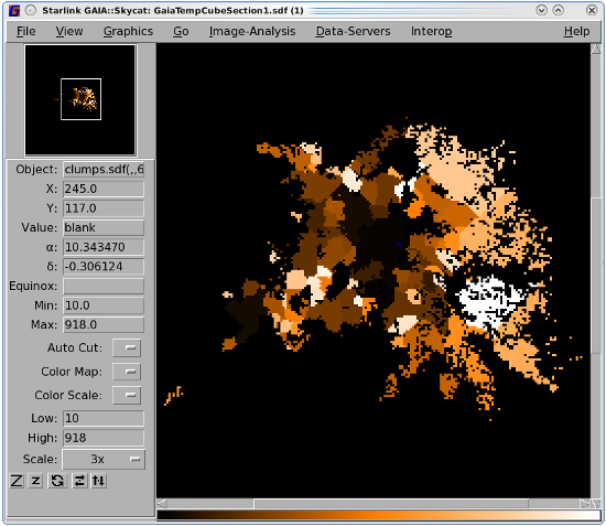
The Cupid application findclumps can be used to generate a clump catalogue. It identifies clumps of emission in one-, two- or three-dimensional NDFs. You can select from the clump-finding algorithms FellWalker, GaussClumps, ClumpFind or Reinhold. You must supply a configuration file which lists the options for whichever algorithm you chose (see the cupid manual for a full list). The result is returned as a catalogue in a text file and as a NDF pixel mask showing the clump boundaries (see Figure 9.2). See Appendix E for descriptions of the various algorithms.
The shape option allows findclumps to create a shape that should be used to describe the spatial coverage of each clump in the output catalogue. It can be set to " None", " Polygon" or " Ellipse". The shape - as described in the output catalogue—is in "STC-S" format. STC-S is a textual format developed by the IVOA for describing regions within a WCS—see here for details.. The STC-S descriptions are added as extra columns to the output catalogue.

| Polygon | Each polygon will have, at most, 15 vertices. For two-dimensional data the polygon is a fit to
the clump’s outer boundary (the region containing all good data values). For three-dimensional
data the spatial footprint of each clump is determined by rejecting the least significant 10% of
spatial pixels, where “significance” is measured by the number of spectral channels that contribute
to the spatial pixel. The polygon is then a fit to the outer boundary of the remaining spatial pixels.
|
|---|---|
| Ellipse | All data values in the clump are projected onto the spatial plane and “size” of the collapsed clump at four different position angles—all separated by 45∘—is found. The ellipse that generates the same sizes at the four position angles is then found and used as the clump shape. |
You can plot the clump outlines over an image using Gaia. See Section 10.4 for instructions.
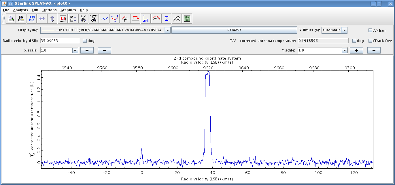
Occasionally you may see unexpected emission within your data. An example is shown in Figure 9.3. In this figure, we use the average spectrum feature (see Section 10.5)—and in this example—we see expected bright emission around 7 km s−1. In addition to the expected bright emission, we see some faint emission around −30 km s−1.

We can use Splat to investigate this emission further (see Section 10.8 on how to open up a spectrum in Splat).
It is possible to use Splat to change the units to Standard of rest: Observer by first going to Analysis and clicking on Change units.
We then use the drop-down menu next to Standard of rest to select Observer from the list, and select Apply.

Now we see the unexpected line is at 0 km s−1, and is therefore likely to be contamination from telluric lines. To confirm a telluric line we can compare the frequency of the unidentified line to the frequency of known telluric lines. To get the frequency of the line again go to Analysis and click on Change units and then change the units to Coordinates: Gigahertz. Finally read off the position of the line.