Processing math: 100%
Chapter 8
Analysing your Cube
8.1 Smoothing your data
Frequency or velocity smoothing is performed using Kappa:block. It uses a rectangular box filter with each
output pixel either the mean or the median of the input pixels within the filter box. The box size can be set to 1
for dimensions which do not require smoothing. In the example below the spatial pixels remain untouched
while the velocity axis is smoothed using a box of five channels.
% block in=mycube out=rebinnedcube box="[1,1,5]"
Two-dimensional NDFs can also be smoothed using gausmooth. This smooths using a symmetrical Gaussian
point spread function (PSF) of specified width(s) and orientation. Each output pixel is the PSF-weighted mean
of the input pixels within the filter box.
% gausmooth in=mymap out=smoothedmap fwhm=3
Note that the fwhm option is given in the number of pixels. For example, to smooth a map with 4′′pixels by a
12′′Gaussian you would set fwhm=3.
8.2 Removing a baseline
Baselines can be removed using Kappa:mfittrend. This routine can fit polynomials up to order 15, or cubic
splines, to each spectrum in your cube. You can specify the ranges to fit via the ranges parameter, or
you can allow them to be determined automatically (auto), say if the number of observations is
large.
% mfittrend in=cube ranges=\"-50 -10 80 160\" order=1 axis=3 out=baselinedcube
If using automatic range determination you should set the numbin option. This is the number of bins in which to
compress the trend line. A single line or average may be noisy so binning is used to improve the signal-to-noise
in order to enhance features that should be masked.
Ideally the bin size should match your line width to get maximum single to noise between the emission and the
background. Be aware that bins that are too big can dilute weaker features. Likewise, bins that are too small will
get noisy at the edges of broad lines. We recommend you experiment with the bin size to find the best fit for
your data.
To exclude features that are not part of the baseline trend you can use the clip option. Use clip
to provide an array of standard deviations for progressive clipping of outliers within each bin.
Once the data have been binned a trend is fit within each bin and the outliers clipped, the
trend is then re-fitted and the outliers again clipped etc. By default this will clip at 2, 2, 2.5 and
3 σ
successively but you may wish to experiment with your own clip levels. The clip option is only used when
auto=true.
For convenience Gaia has a Baseline tab in its cube control panel—see Section 10.1 for an example. This
invokes mfittrend.
8.2.1 Advanced method
These steps give a more in depth way of determining the baselines and mimic the pipeline.
-
(1)
- Perform a block smooth on your reduced cube. Here the smoothing is quite aggressive with a box filter of
five pixels along the spatial axes and fifteen pixels along the frequency axis. This is to really pull out all
emission features. You can tweak these to suit your data, e.g a narrower box might be needed if you have
very narrow lines.
% block in=cube out=temp1 box="[5,5,15]" estimator=mean
-
(2)
- Perform mfittrend on your smoothed cube with a high-order polynomial and automatic range
determination.
% mfittrend in=temp1 out=temp2 axis=3 order=3 auto method=single \
variance subtract=false mask=blmask
-
(3)
- Add the baseline mask to your original unsmoothed cube.
% add in1=cube in2=blmask out=temp3
-
(4)
- Perform mfittrend on your masked unsmoothed cube with a lower-order polynomial. This time fit the full
range by setting
auto=false.
% mfittrend in=temp3 out=temp4 axis=3 order=1 auto=false ranges=\! \
method=single variance=true subtract=false
-
(5)
- Subtract the baseline from the original unsmoothed cube.
% sub in1=cube in2=temp4 out=baselinedcube
8.2.2 What about findback?
The Cupid routine findback offers an alternative for background subtraction however there are more
limitations. It applies spatial filtering to remove structure with a size scale less than a specified box size. Within
each box the values are replaced by the minimum of the input values. The data are then filtered again and this
time replaced with the maximum in each box.
Using findback results in a baseline trend that hugs the lower limit of the noise and can contain
sharp edges. These problems can be mitigated but extra steps are required. See SUN/255 for more
details.
8.3 Collapsing your map
An integrated intensity map can be created by collapsing your cube along the frequency/velocity axis using
Kappa:collapse. For each output pixel, all input pixels between the specified bounds are collapsed and
combined using one of a selection of estimators. Amongst others, the estimators include the mean, integrated
value, maximum value, the mean weighted by the variance, RMS value and total value. See SUN/95 for a full
list.
The example below includes the options low and high which can be specified to
limit the range over which the cube is collapsed on the given axis (in this case from
−5 km s−1 to
+10 km s−1).
The variance flag indicates the variance array should be used to define weights and generate an output
variance. The option wlim sets the fraction of pixels that must be ‘good’ in the collapse range for a valid output
pixel to be generated. You may find you need to reduce the value for wlim below its default of 0.3 for some
data.
% collapse in=cube axis=vrad estimator=integ variance=true low=-5.0 high=10.0 \
wlim=0.5 out=integmap
If you do not know the axis name you can give the number instead (1=RA, 2=Dec, 3=vrad).
For convenience Gaia has a Collapse tab in its cube control panel—see Section 10.6 for an example. This
invokes collapse.
8.3.1 Advanced method
These steps mimic the pipeline and show the procedure for generating an integrated map collapsed only over regions with
emission greater than 3 σ.
-
(1)
- Use findclumps to run a clump-finding algorithm on your cube. Specify the
3 σ
limit in your configuration file. See Section 9.5 for more details on clump-finding and Section 8.9 for how
to determine your RMS.
% findclumps in=cube rms=<medianrms> config=^myconfig.dat \
method=clumpfind out=temp1 outcat=mycat deconv=no
-
(2)
- Divide the map by itself to create a clump mask that has clump regions set to 1.
% div in1=temp1 in2=temp1 out=temp2
-
(3)
- Set the bad data to zero using Kappa:nomagic.
% nomagic in=temp2 out=temp3 repval=0
-
(4)
- Multiply your reduced cube by the clump mask.
% mult in1=cube in2=temp3 out=maskedcube
-
(5)
- Collapse your masked reduced cube.
% collapse in=maskedcube out=integ estimator=integ wlim=0.1 variance
8.3.2 Moments maps
You can use collapse to generate the moments maps by selecting the appropriate estimator option—Integrated
value (Integ) for the integrated map (zeroth moment), Intensity-weighted co-ordinate (Iwc) to get the velocity
field (first moment), or Intensity-weighted dispersion (Iwd) to get the velocity dispersion (second
moment).
Tip: You can also use the
Picard recipe CREATE_MOMENTS_MAPS. See Appendix
A for details. This recipe
follows the advanced method outlined above.
8.4 Temperature scales
Your cube will come out of makecube and the pipeline, in units of
T∗A. To convert this to main-beam
brightness temperature, TMB divide your
cube by the main-beam efficiency, ηMB.
Alternatively, to convert to corrected radiation temperature,
T∗R, divide by the forward scattering
and spillover efficiency, η fss.
See Section 3.2 for efficiency values for RxA and HARP, and the JCMT webpages for further information and
historical numbers.
You can use the Kappa command cdiv to divide any NDF by a constant.
% cdiv in=harpcube scalar=0.63 out=harpcube_Tmb
8.5 Changing the pixel size
You may want to regrid your data onto larger pixels, for instance to allow direct comparison with data from
other observatories. In the example below a JCMT map is regridded and aligned to match a Herschel map. See
Appendix B for instructions on converting your FITS file to NDF format.
% wcsalign in=jcmtmap out=regridmap lbnd=! ubnd=! ref=herschelmap rebin conserve=f
Alternatively, to resample your data onto smaller pixels you should use the Kappa command sqorst. In the
example below ’map’ has a pixel size of 8′′, while ‘resamplemap’ has a pixel size of 4′′– the number of pixels has
been doubled by applying a factor of 2 to the spatial axes. A factor of 1 was applied to the frequency (third) axis
leaving it unchanged.
% sqorst in=map out=resamplemap factors="[2,2,1]" conserve
mode=factors is the default setting so it was not specified in the example above. The example below however,
uses mode=pixelscale to define a pixel size for the third axis; here the spectra are rebinned into
2 km s−1 channels.
% sqorst in=map out=resamplemap mode=pixelscale pixscale=2 axis=3
Remember you can check your current pixel size and channel spacing with ndftrace (see Section 2.4).
8.6 Mosaicking cubes
If you pass raw files covering different regions of the sky to makecube it will automatically mosaic
them together. This can be heavy work for your processor so you may wish to make individual
cubes and combine them during post-processing. To co-add multiple reduced maps you should use
wcsmosaic.
Note that this is not the same as stitching the tiles of a reduced cube from a single makecube command. Such
tiles share common pixel co-ordinates and so can be combined with paste (Section 6.6.1). Separately created
cubes will not have the same pixel co-ordinates, and therefore the world co-ordinates are required to align the
tesserae in the mosaic of an extended region.
% wcsmosaic in=^maplist out=mosaic lbnd=! ubnd=! variance
By selecting the lower bound (lbnd) and upper bound (ubnd) to be default (!) you are including all of the input
tiles. You can change these if you want to only mosaic a sub-region of the input maps. As with makecube there
are a number of regridding options available to you describing how to divide an input pixel between a group of
neighbouring output ones (the default is SincSinc).
Note that by default wcsmosaic aligns reduced cubes along the spectral axis using the heliocentric standard of
rest (the Orac-dr pipeline also does this). If you want to align using a non-heliocentric standard of rest, you
should set the AlignStdOfRest attribute for your NDFs using wcsattrib before running wcsmosaic. The following
example sets the alignment to the kinematic LSR.
% wcsattrib <list_of_separate_cubes> set AlignStdOfRest LSRK
where <list_of_separate_cubes>
is group of cubes specified as a comma-separated list or as one per line in a text file.
Tip: Take care not to combine data separated on the sky as
wcsmosaic will attempt to create a vast cube that
encompasses all the input files until it runs out of resources.
Tip: You can also use the
Picard recipe MOSAIC_JCMT_IMAGES. This will correctly combine all NDF
extensions. See Appendix
A for details.
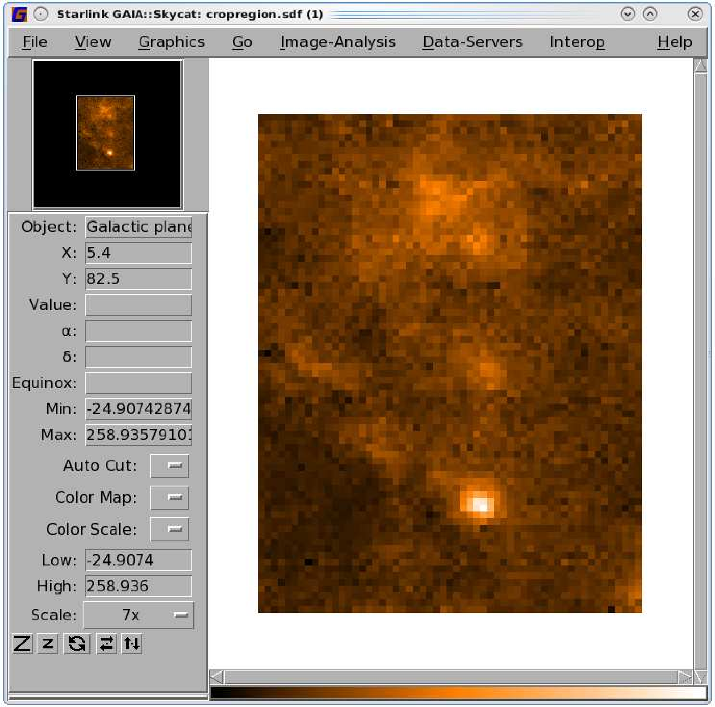
8.7 Cropping your map
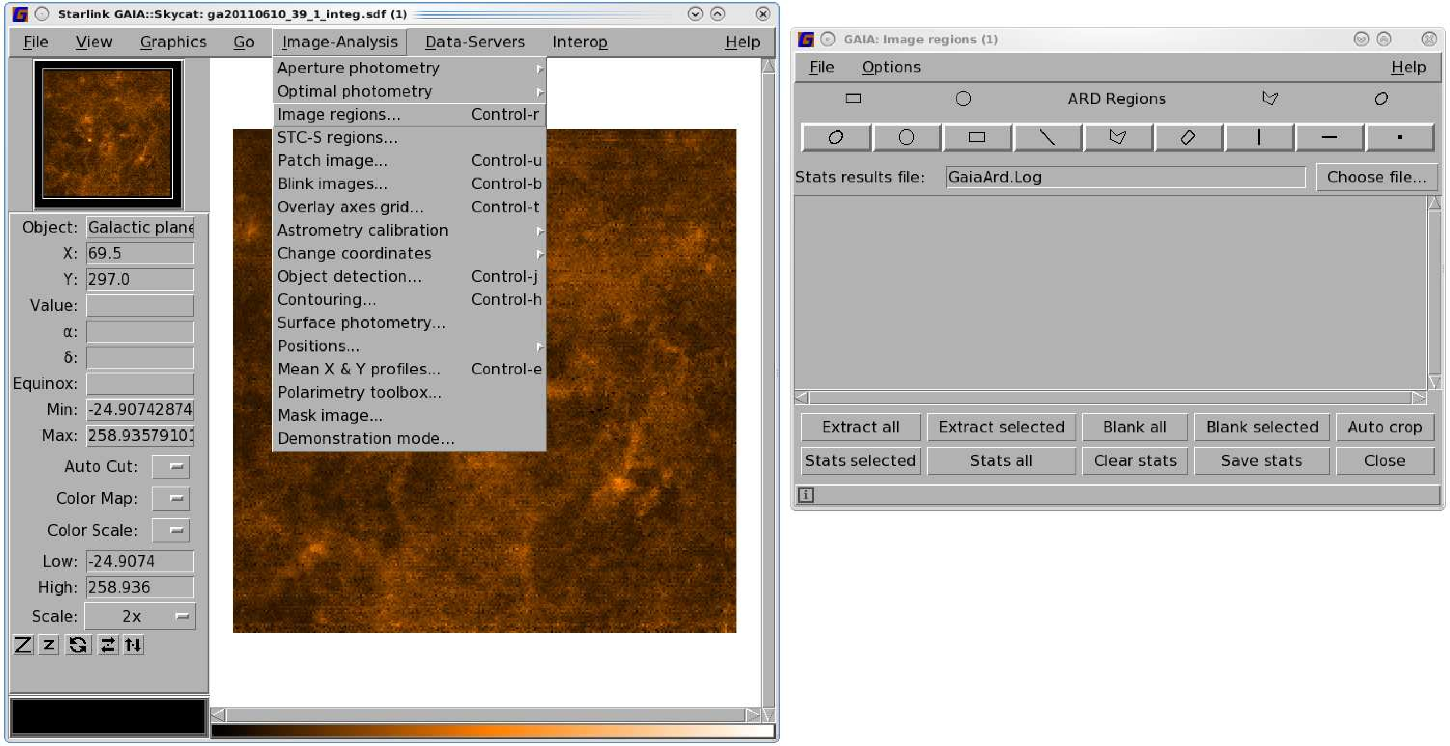
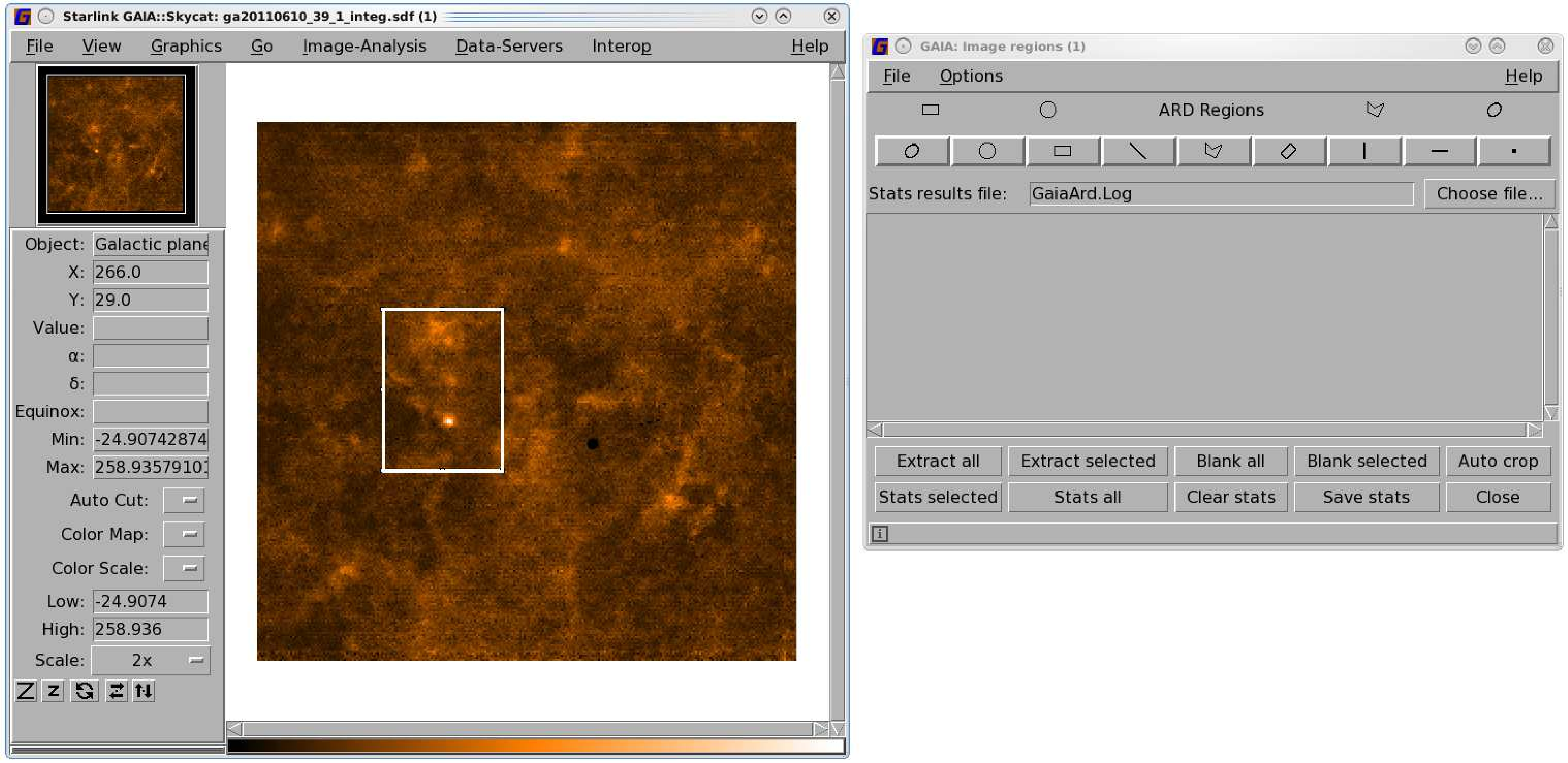
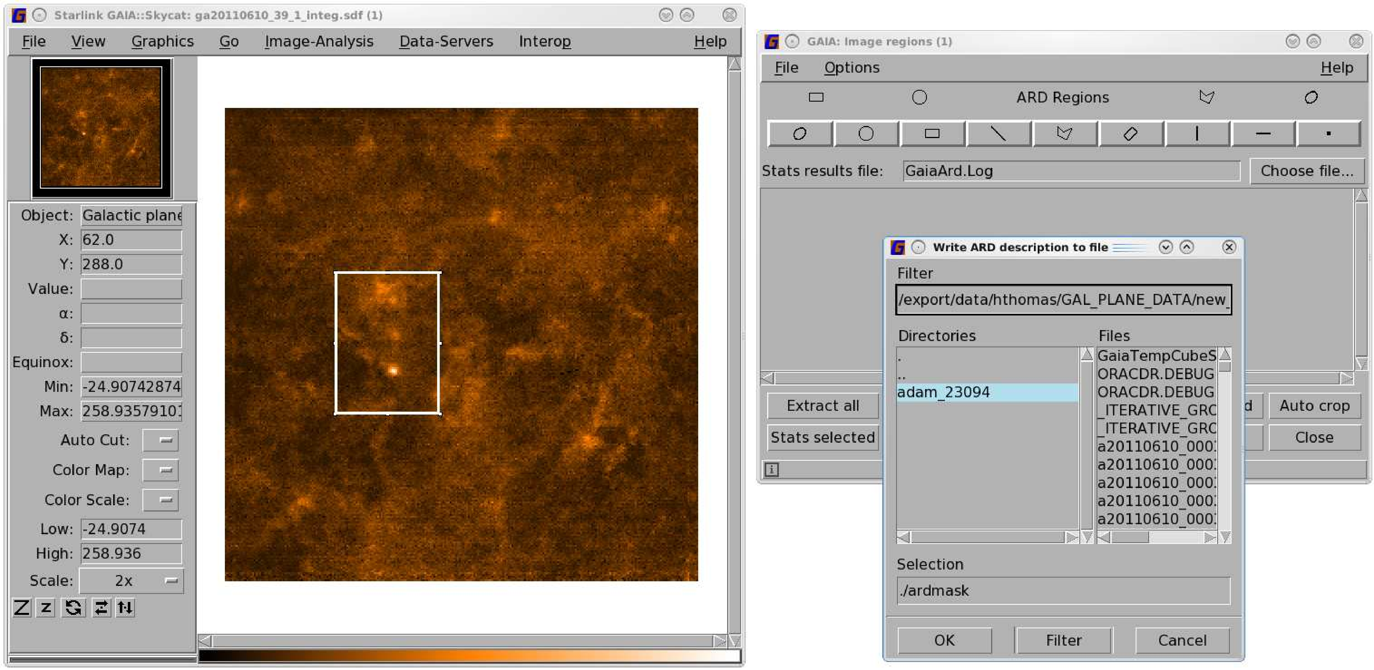
Cropping an ACSIS map can be fiddly. The simplest way is to create an ARD mask in Gaia and apply it to your
map. The steps below work on both two- and three-dimensional data.
-
(1)
- Create your ARD mask. You may find it easiest to do this with Gaia. See Figure 8.2 for an
illustrated guide.
-
(2)
- Trim off the third axis from your mask using ndfcopy.
% ndfcopy mask trim trimwcs
-
(3)
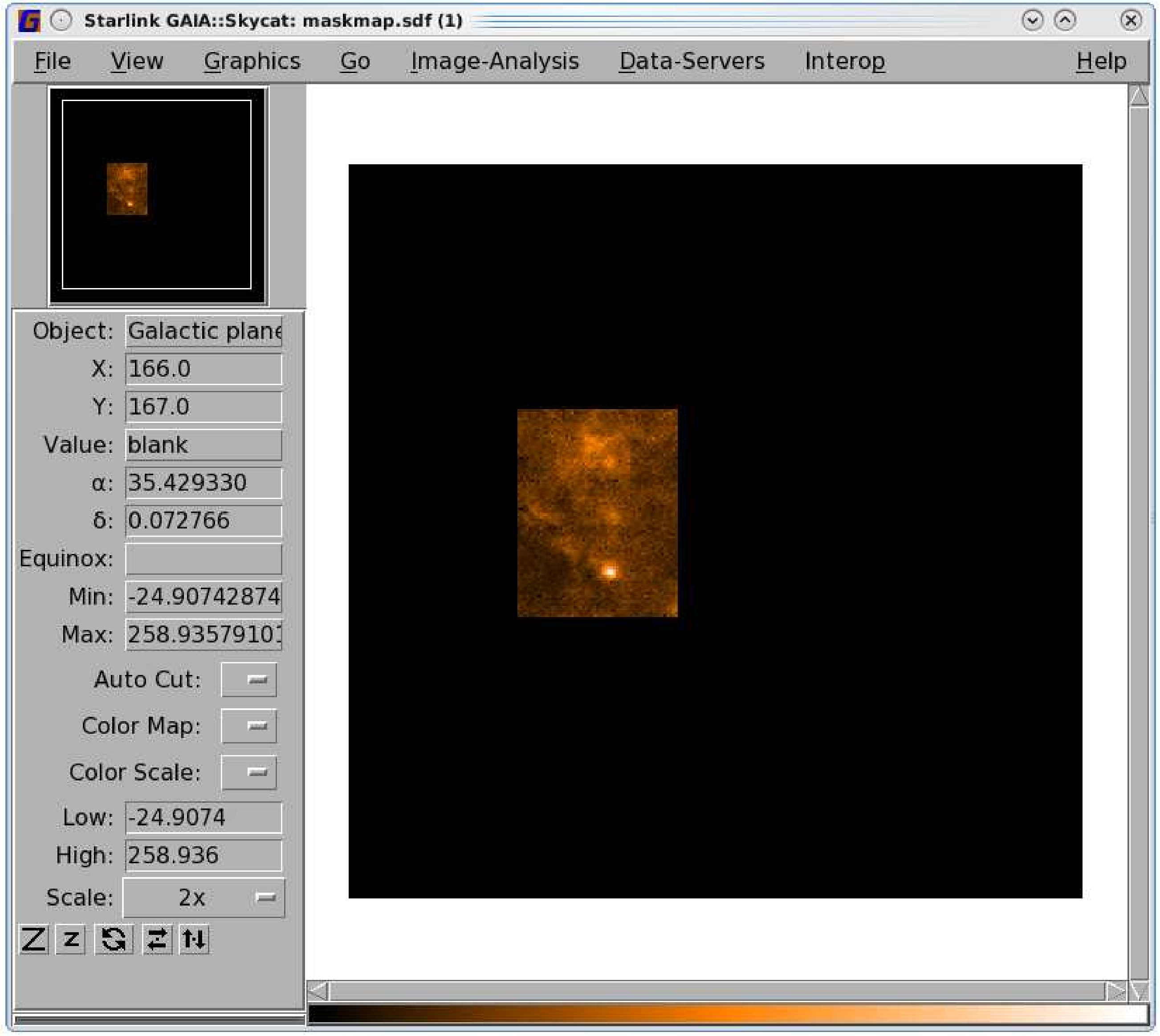
- Apply the saved ARD mask to your map. Setting
inside=false will mask the pixels outside rather than
inside your mask. The masked pixels will appear blank when you open it with Gaia; see the left-hand
panel of Figure 8.2.
% ardmask map inside=false ard=ardmask.txt out=maskmap
-
(4)
- Trim off the blank pixels using ndfcopy with the
trimbad option. This leaves just your selected region; see
the right-hand panel of Figure 8.2.
% ndfcopy maskmap trimbad
An alternative method is to use ndfcopy while defining the section of the map or cube you wish to extract as an
output cube. See Section 2.6.
8.7.1 Supplying a template
If you wish to extract only a region which overlaps with an existing file you have, e.g. from a different observing
campaign or telescope, you can also use ndfcopy but with the like option.
% ndfcopy in_full out_cropped like=map2 likewcs
The shape of the file supplied by like will determine the shape of the output file. This shape can be in either
pixel indices or the current WCS Frame. If the WCS Frame is required, include the parameter likewcs to the
command line otherwise it can be omitted.
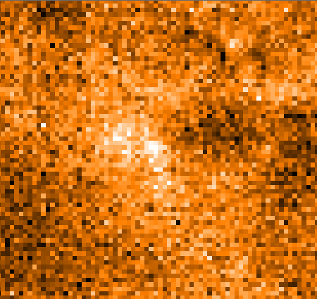
8.8 Filling holes in your map
You may come across empty pixels in your map due to dead receptors or receptors which have failed quality
assurance in the pipeline. The second half of 2013 in particular had only twelve working receptors for
HARP.
You can fill these holes using Kappa:fillbad. This replaces the bad values with a smooth function derived from
neighbouring values, derived by iterating to a solution of Laplace’s equation.
The default values for fillbad will fill the holes but smooths by five pixels along
each axis. If you prefer not to smooth in the spectral axis, set the parameter size to
[s,s,0]
where s
is the scale length in pixels. The zero means do not smooth along the third axis.
The scale length should have a value about half the size of the largest region of bad data to be replaced.
Since the largest bad regions apart from the cube peripheries are two pixels across, a size of 1 is
appropriate.
% fillbad in=holeymap out=filledmap size="[1,1,0]"
Figure 8.3 shows an initial map with holes and the final filled map.
8.9 Checking the noise
You can use Kappa:stats to check the noise in your map. It will report the statistics for all pixels so be aware that
noisy edges and strong signal will contribute to the standard deviation. You can mitigate this by trimming any
noisy edges and by examining the square root of the VARIANCE component (hereafter referred to as the error
component)
although bright emission will still increase your noise. You can select the error component with comp=err on the
command line.
% stats file comp=err order
Including the option order allows the ordered statistics such as the median and percentiles to be reported. Note
that percentile options will need to be specified via the percentiles parameter.
Tip: Remember the mean or median values will give you the noise when using the error component.
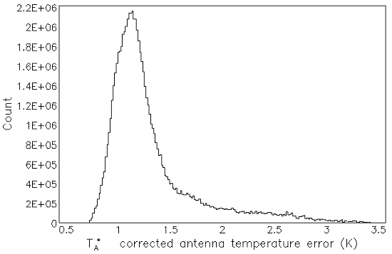
8.9.1 Visualising the noise
You can plot the noise or error component of your map using the Kappa command histogram. This allows you
to visualise the distribution with more ease. Again the comp=err option is used.
% histogram mosaic comp=err range=! numbin=200
The output is shown in Figure 8.4. An alternative to setting the number of bins via the numbin parameter is to
set the width of each bin using the width parameter.
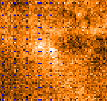
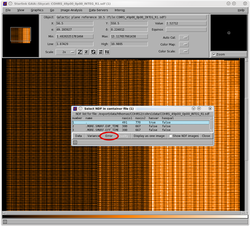
It is also useful to view the noise map itself. Figure 8.5 shows how to select the error component in Gaia. Other
options available from the "Select NDF in container file" window include the exposure time, the effective
time and, if spread=nearest when running makecube, the system temperature. To return to your main image
select the top level and click the Data button.
Tip: You can write out the error component into a new file using
ndfcopy.
% ndfcopy map comp=err noisemap
8.9.2 HARP flatfielding
The individual detectors in the HARP array do not respond exactly the same to the incoming signal, returning
different temperatures for the same flux. If uncorrected, this can lead to artificial net-like patterns in the reduced
spectral cube. As with any flatfield correction, the goal is to expose to a uniform source to measure the relative
responses of the detectors. However, this is not possible with HARP observations, and the approach is assume
that during an observation the detectors see approximately the same signal from the various sources. For
extended emission at low galactic latitudes this is a reasonable assumption. For isolated compact sources it is
likely to be invalid.
It may be possible to use a flatfield determined on the same night in a high-signal region and apply that to a
low-signal or compact-source observation. The flatfield can change during the night, but it might better than no
flatfield.
The method of Curtis et al. (2010)[9] creates a map for each detector and integrates the measured
flux in the main spectral line. Use the DETECTORS parameter to create a spectral cube from just that
detector.
% makecube in=rawfile out=cube_H01 detectors="’H01’" autogrid
The simplest way to sum the flux across a line run stats over a chosen spectral range, such as
−5 km s−1 to
7.2 km s−1.
% stats cube_H01"(,,-5.0:7.2)"
If there might be bad pixels present, the mean is more accurate than the sum. This assumes that the
line is located within these bounds across the whole spatial region. It is wise not to push too far
into the wings of the line and baseline errors and noise have a greater impact on the integrated
flux.
The receptors are normalised to the flux of the reference receptor, near the centre, normally H05, but given by
the FITS header REFRECEP.
There are other methods in Orac-dr, one to cope with multiple lines. It sums all the signal above some threshold,
such as the median plus four standard deviations, to exclude the baseline noise. Since the flat ratio biases this
sum, Orac-dr iterates to converge to a solution.
Copyright © 2015-2021 Science and Technology Facilities Council,
& East Asian Observatory