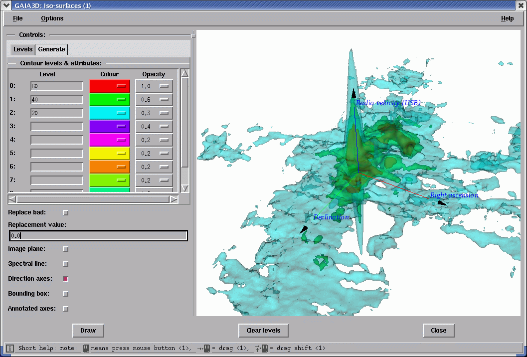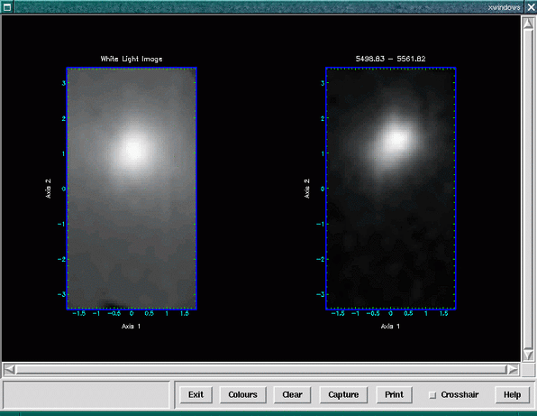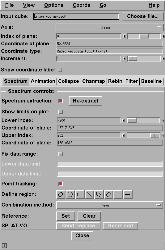
Figure 2: The Gaia toolbox for displaying a cube.
While the initial data-reduction software for IFUs is highly instrument dependent, the data analysis of the final science data product for all these instruments should be fairly generic. The end product of the data reduction for IFS is, almost naturally, an x,y,λ data cube. For instruments not working in the optical and infrared regimes, the third axis may also be in some other spectral co-ordinate system, such as frequency. Once assembled, with associated variance and quality arrays, scientifically interesting information can be extracted from the cube.
For long-slit paradigm instruments a data cube is the only data product available, as overlapping
point-spread functions mean that the spectral data must be resampled. For MOS paradigm data, while
the individual spectra are available, data visualisation is often intrinisically more intuitive if done on
resampled data cubes. As such, this cookbook will (in the main) only deal with applications that handle
the data-cube format. If you have already sourced the Starlink /star/etc/login and /star/etc/cshrc
files1
then the commands kappa, figaro, and ccdpack will set up access to the Kappa, Figaro, and
Ccdpack tasks respectively, including most of the following applications.
Some of the most fundamental operations you might wish to perform on a data cube are the arithmetic operations of addition, subtraction, multiplication and division, both by scalars and other data cubes. All these basic operations, and additional more complicated ones, can be carried out using tasks from the Kappa package. Detailed documentation for all of these tasks can be found in SUN/95.
Slightly more complex is manipulation and resampling of the data cube itself. The most important utilities available to do this within Kappa are the collapse, chanmap, ndfcopy, and pluck applications. collapse can produce white-light and passband images (see Section 5.8) and velocity maps by the appropriate selection of statistic. chanmap creates a grid of passbands. ndfcopy can extract a single spectrum (along pixel axes) or arbitrary cube sections (again see Section 5.8 for details), while pluck uses interpolation to extract at arbitrary positions, such as a spectrum at nominated equatorial co-ordinates, or an image at a given wavelength or frequency. Some applications require the spectral axis to be the first or the third axis; permaxes allows shuffling of the pixel axes.
While IFU data is intrinsically three dimensional there are times when it is necessary to deal with two dimensional images during analysis (e.g. velocity maps). Some potentially useful Kappa applications which are restricted to handling two-dimensional files are
Some tasks operate in two dimensions, but apply processing to a series of planes in a cube. They permit, for example, to smooth spatially while retaining the spectral resolution.
There are several applications which can carry out operations on individual pixels, the most general of these is chpix which can replace the pixel value of a single, or region, of pixels with an user defined value (including the bad magic value).
Building processing scripts from the Starlink applications can involve you manipulating or querying information about structures within the NDF file itself, three useful Kappa commands to do this are listed below.
In some cases NDF information must be modified after a processing step (e.g. the NDF title) or, in the case of a newly created NDF (see Section 6.6), we must generate inital values. Kappa provides various tools to manipulate NDF extensions.
Combined with the graphics devices commands (see Section 5.3) the following applications, especially clinplot, display, linplot and contour act as the backbone for image display, and some complex effects can be generated using these elemental tasks.
Mosaicking multiple IFU data cubes together is something you may well wish to consider, unfortuantely there are problems involved in doing so (see Section 5.9), however, the following tasks from Kappa may be useful
along with the following tasks from Ccdpack.
Some of the most useful applications available for spectral fitting and manipulation live inside Figaro as part of SPECDRE. Some of these applications work on individual spectra, however, others read a whole cube at once and work on each row in turn. A possible problem at this stage is that many of these applications expect the spectroscopic axis to be the first in the cube, whereas for the current generation of IFU data cubes the spectral axis is typically the third axis in the cube. Kappa permaxes can reconfigure the cube as needed by the various packages. A full list of SPECDRE applications can be found in SUN/86.
One of the fundamental building blocks of spectral analysis is gaussian fitting, amougst other tools, Figaro provides the fitgauss application (part of SPECDRE) to carry out this task.
FITGAUSS is especially well suited to automation inside a script. For example,
we call the fitgauss routine here specifying all the necessary parameters, and suppressing user interaction, to allow us to automatically fit a spectrum from inside a shell script. Here we have specified an input file, ${spectrum} and the lower and upper boundaries of the fitting region, ${low_mask}, and ${upp_mask}, respectively. Various initial guesses for the fitting parameters have also been specified: the continuum level ${cont}, peak height ${peak}, full-width half-maximum ${fwhm} and the line centre ${position}. By specifying ncomp=1 cf=0 pf=0 wf=0 we have told the application that we want it to fit a single gaussian with the central line position, peak height and FWHM being free to vary.
In addition we have turned off user interaction with the application, by setting the following parameters, reguess=no, remask=no, dialog=f and fitgood=yes.
This allows fitgauss to go about the fit without further user intervention, displaying its resulting fit in
an X-display, logging the fit characteristics to a file (${fitfile}) and saving the fit in the SPECDRE
extension (see SUN/86 for details) of the NDF where it is available for future reference and
manipulation by other SPECDRE applications.
The velmap and peakmap scripts are based around the SPECDRE fitgauss application.
For data with a significantly varying continuum mfittrend is available in Kappa to fit and remove the continuum signal, thereby making fitgauss’s job easier.
The ability to identify and measure the properties of features can play an important role in spectral-cube analysis. For example, you may wish to locate emission lines and obtain their widths as initial guesses to spectral fitting, or to mask the lines in order to determine the baseline or continuum. Extending to three dimensions you may want to identify and measure the properties of clumps of comoving emission in a velocity cube. The Cupid package addresses these needs.
The findclumps is the main command. It offers a choice of clump-finding algorithms with detailed configuration control, and generates a catalogue in FITS format storing for each peak its centre and centroid co-ordinates, its width, peak value, total flux and number of contributing pixels. Information from the catalogue can be extracted into scripts using STILTS and in particular its powerful tpipe command.
Here we find the clumps in the three-dimensional NDF called cube using the configuration stored in
the text file ClumpFind.par that will specify things like the minimum number of pixels in a clump, the
instruments’s beam FWHM, and tuning of the particular clump-finding algorithm chosen. The
PERSPECTRUM parameter requests that the spectra be analysed independently. It would be absent if
you were looking for features in a velocity cube. The contents of output NDF clumps is algorithm
dependent, but in most cases its data array stores the index of the clump in which each pixel resides,
and all contain clump information and cut-outs of the original data about each clump in
an extension called CUPID; and its QUALITY array has flags to indicate if the pixel is
part of a clump or background. The last is useful for masking and inspecting the located
clumps.
Some experimentation with findclumps algorithms and configuration to obtain a suitable segmentation for your data’s characteristics is expected. That is why we have not listed any configuration parameters or even chosen a clump-finding algorithm in the example.
Continuing with the example, the catalogue of clumps detected and passing any threshold criteria are
stored in cubeclump.FIT. (See the Cupid manual for details of all the column names.) We then use
tpipe to select the third axis centroid co-ordinate (Cen3) of the first clump (index==1) and store the
numerical value in shell variable peak. The commands cmd= are executed in the order they
appear.
This could be extended to keep other columns keepcols and return them in an array of the line with
most flux given in column Sum.
Here tpipe sorts the fluxes, picks that clump, and writes an ASCII catalogue containing the
centroid and width along the third axis storing the one-line catalogue to shell variable
parline. In this format the names of the columns appear first, hence the required values are
in the third and fourth elements. We could have used the csv-nohead output format to
give a comma-separated list of values as in the previous example, and split these with
awk.
tpipe has many command options that for example permit the selection, addition, and deletion of columns; and the statistics of columns. The selections can be complex boolean expressions involving many columns. There are even functions to compute angular distances on the sky, to say select a spatial region. See the STILTS manual for many examples.
Cupid also includes a background-tracing and subtraction application findback. You may need to run this or mfittrend to remove the background before feature detection. Note the if you are applying findback to the spectra independently, the spectral axis must be first, even if this demands a re-orient the cube.
In this example, the spectral axis is the third axis of NDF cube. findback removes structure smaller
than $box pixels along each spectrum independently. The resulting estimated backgrounds for each
spectrum are stored in NDF backperm, which is re-oriented to the original axis permutation to allow
subtraction from cube.
Kappa and other Starlink applications using PGPLOT graphics have a single graphics device for line and image graphics. These can be specified as either PGPLOT or Starlink device names. The current device may be set using the gdset command as in the example below.
You can use the gdnames command to query which graphics devices are available, and your choice of device will remain in force, and can be inspected using the globals command, e.g.
unless unset using the noglobals, or overriden using the DEVICE parameter option in a
specific application. Predicatably, the gdclear command can be used to clear the graphics
device.
More information on these and other graphics topics can be found in SUN/95.
Each Starlink application which makes use of the standard Starlink graphics calls, which is most of them, creates an entry in the graphics database. This allows the applications to interact, for instance you can display an image to an X-Window display device using the display command, and later query a pixel position using the cursor command.
The graphics database is referred to as the AGI database, after the name of the subroutine library used to access its contents, and exists as a file stored in your home directory. In most circumstances it will be named for the machine you are working on.
An extensive introduction sprinkled with tutorial examples to making full use of the graphics database can be found in the Kappa manual (SUN/95) in the sections entitled The Graphics Database in Action and Other Graphics Database Facilities. There is little point in repeating the information here, however learning to manipulate the graphics database provides you with powerful tools in visualising your IFU data, as well as letting you produce pretty publication quality plots. For instance, the compare shell script make fairly trivial use of the graphics database to produce multiple image and line plots on a single GWM graphics device.
The different display types, such as pseudo colour and true colour, are explained in detail in the Graphics Cookbook (SC/15).
On pseudo-colour displays Kappa uses a number of look-up tables (commonly refered to as LUTs) to manipulate the colours of your display. For instance you may want to have your images displayed in grey scale (lutgrey) or using a false colour ‘heat’ scale (lutheat). Kappa has many applications to deal with LUTs (see SUN/95), these applications can easily be identified as they all start with “lut”, e.g. lutable, lutcol.
World Co-ordinate System (i.e. real world co-ordinates) information is a complex topic, and one that many people, including the author, find confusing at times.
Starlink applications usually deal with WCS information using the AST subroutine library (see SUN/210 for Fortran and SUN/211 for C language bindings), although notably some parts of Figaro (such as SPECDRE) have legacy and totally independent methods of dealing with WCS information. See Section 6.6 for an example of how to overcome this interoperability issue.
This general approach has an underlying effect on how Starlink applications look at co-ordinate systems and your data in general.
Starlink applications therefore tend to deal with co-ordinate ‘Frames’. For instance, the PIXEL Frame is the frame in which your data is considered in the physical pixels with a specified origin, i.e. for a simple two-dimensional example, your data frame may have an x size of 100 pixels and a y size of 150 pixels with the origin of the frame at the co-ordinates (20,30). Another frame is the SKY frame, which positions your image in the real sky—normally right ascension and declination but other sky co-ordinate systems are available and easily transformed. A ‘mapping’ between these two frames will exist, and will be described, inside the WCS extension of your NDF. The Kappa wcscopy application can be used to copy WCS component from one NDF to another, optionally introducing a linear transformation of pixel co-ordinates in the process. This can be used to add WCS information back into an NDF which has been stripped of WCS information by non-WCS aware applications. Further details about WCS Frames are available in SUN/95 Using World Co-ordinate Systems.
Why is this important? Well, for instance, the display command will automatically plot your data with axes annotated with co-ordinates described by the current WCS frame, so if your data contains a SKY frame it can (and much of the time will) be automatically be plotted annotaed with the real sky co-ordinates, usyally right ascension and declination, of the observation. It is also critical for mosaicking of data cubes, as explained later in Section 5.9.
Both Kappa and Ccdpack contain commands to handle WCS NDF extensions. In Kappa we have the following applications.
while Ccdpack has
which is a very useful utility for handling frames within the extension. For instance,
here we see that ifu_file.sdf has three WCS frames, the base GRID frame with origin (1,1,1), a
PIXEL frame with origin (0.5,0.5,0.5) and an AXIS frame with real world co-ordinate mapped on to the
PIXEL frame.
ndftrace also contains a useful option at this point: FULLFRAME. In the following example, most of the
ndftrace output is excised for clarity, denoted by a vertical ellipsis.
The important information here is the boundary of the image in the PIXEL and CURRENT frame of the NDF, the CURRENT frame being the current ‘default’ frame which applications accessing the NDF will report co-ordinates from (the CURRENT frame of the NDF can be changed using the Kappa wcsframe command and is usually the last accessed frame in the extension). In this case we can see that the current frame is the SKY-SPECTRUM frame, with extent 5:36:51 to 5:36:53.0 in right ascension, −7:26:14 to −7:25:44 in declination, and 345.762 to 345.8139 Ghz in frequency.
Gaia is a display and analysis tool widely used for two-dimensional data. For many years the
Gaia tool had little to offer for cube visualisation. At the appropriately named Version 3.0, came a
toolbox for cubes to permit inspection of planes individually, or as an animation, or as a passband
image by collapsing. Now at the time of writing, Version 4.2 Gaia offers further facilities,
such as rendering, for cube analysis. Gaia is also under active delevopment. Check the
$STARLINK_DIR/news/gaia.news file for the latest features extending upon those summarised
below.
If you start up Gaia with a cube
the cube toolbox appears (see Figure 2). In the upper portion you may choose the axis perpendicular to the axes visible in the regular two-dimensional display; this will normally be the spectral axis, and that is what is assumed this manual. You can select a plane to view in the main display by giving its index or adjusting the slider.The lower portion of the toolbox has a tabbed interface to a selection of methods. The controls change for each method. Of particular note are the following methods.
Animation tab Spectrum tab Collapse tab Iwc gives a form of velocity map, and Iwd estimates the line dispersions.
Chanmap tab Rebin tab Filter tab If you need to access the Cube toolbox, go to the Open cube... option in the File menu of the main
display.
Once you have an image displayed, be it a plane, passband image or channel map, you can then use
Gaia’s wide selection of image-display facilities described in SUN/214 (also see SC/17) to enhance the
elements under investigation. There are also many analysis capabilities mostly through the
(Image-Analysis menu), including masking and flux measurement.
One of the most useful facilities for cube analysis is a dynamic spectrum display. Once you have a
representative image displayed, click on the mouse over the image a line plot along the spectral axis
appears. As you drag the cursor holding down the first mouse button, the spectrum display updates
to dynamically to reflect the current spatial location while the data limits are unchanged. If you click again
the range will reset to the current spectrum. You can enforce autoscaling as you drag too by enabling
Options→Autoscale
in the spectral plot’s control bar. This is slower although it allows an intensity independent
comparison of the spectra. The Spectrum tab mentioned earlier also allows control of the plotting
range along both axes. The Reference: Set button lets you nominate the current spectrum as a
reference spectrum. Then as you subsequently drag the mouse you can compare any of the spectra
with the reference spectrum. See Figure 3.
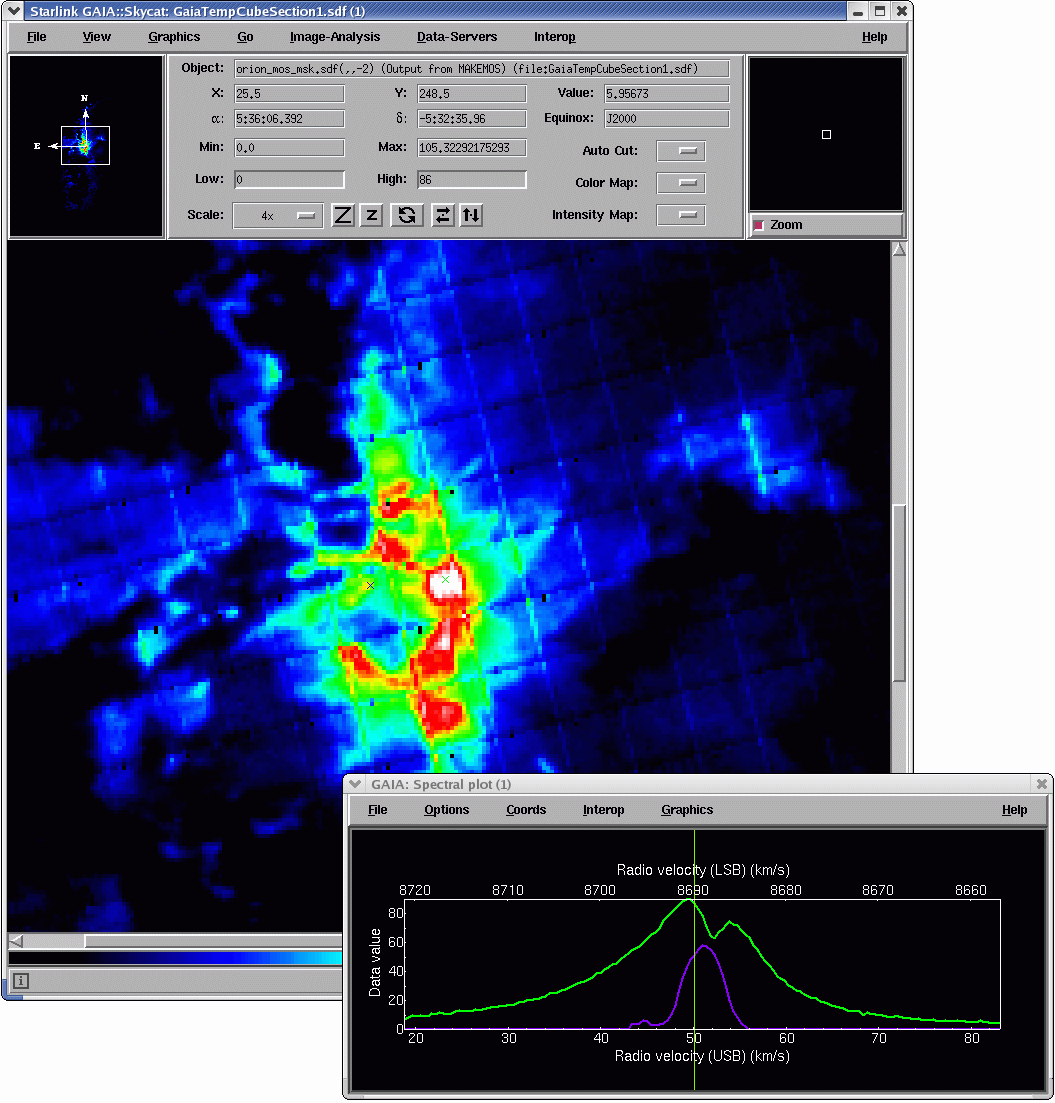
The vertical red line shows the plane being displayed in the main viewer. You can drag that line with the mouse to adjust the plane on view, say to inspect where emission at a chosen velocity lies spatially.
Further features of the spectral viewer can be found in the online help.
The View menu in the cube toolbox offers two interactive rendering functions that let you explore your
cube in three dimensions.
The first of these is iso-surface. It’s akin to contouring of an image extended to three dimensions. Each coloured surface corresponds to a constant data value. In order to see inside a surface, each surface should have an opacity that is less than 1.0. An example using the same Orion dataset is in Figure 4.
Just as with the contouring in Gaia, there are different methods to generate iso-surface levels authomatically, as well as manually.
You can adjust the viewing angle and zoom factor either with the mouse, or with the keyboard for finer control. The online help lists the various controls. There are many options to control the appearance, such as directional and annotated axes. Gaia can also display the current slice and displayed spectrum. It is also possible to display two cubes simultaneously, say to compare data from different wavelengths measuring different molecular species. Gaia provides a number of alignment options in this regard.
The second function is volume rendering. It displays all the data within two data limits as a single volume. You assign a colour and opacity to each limit. The controls and options are the same as for the iso-surfaces. See Figure 5.
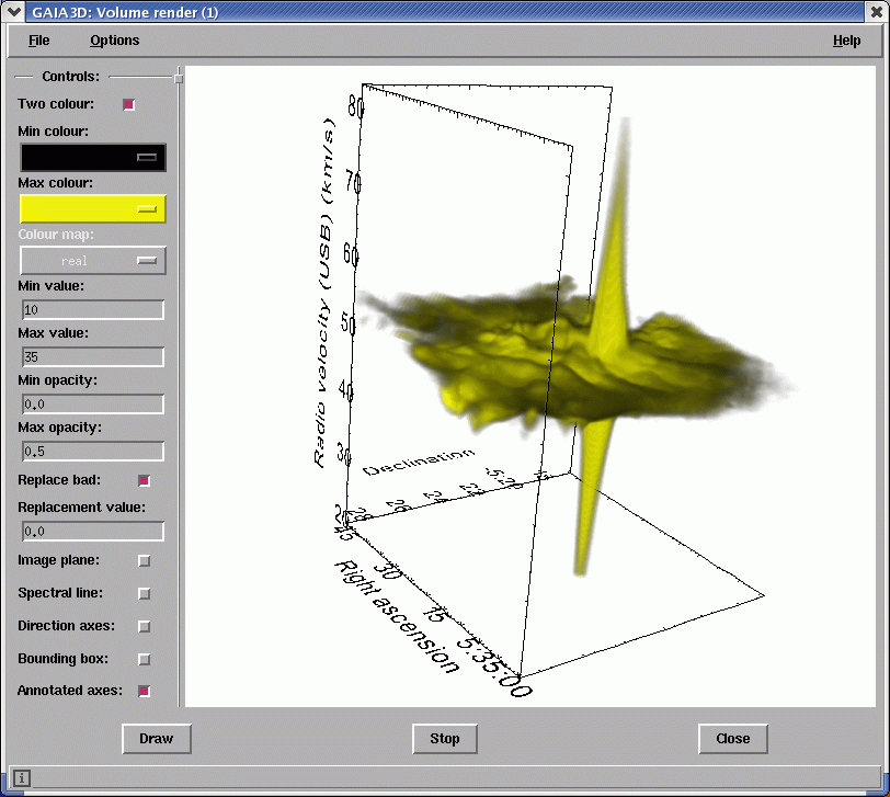
These visualisation functions place heavy demands on computer memory and CPU. Also a modern graphics card with hardware support for OpenGL makes a huge difference in interactive performance. So you will need a modern machine to get the best out of these tools. Of the two tools, iso-surface is quicker to render and uses less memory.
IDL has extensive visualisations capabilities and has many of the tools needed to analyse IFU data cubes available ‘off the shelf’. Unfortunately, due to the large file sizes involved, some of the more useful tools availble in IDL can be very slow on machines with small amounts (<512 Mb) of memory.
Like many modern UNIX applications IDL suffers problems coping with pseudo and true colour displays. When writing IDL scripts it is important to bear in mind the display type you are using, for pseudo colour (8 bpp) displays you should set the X device type as follows
while for true-colour displays, commonly found on modern machines running Linux, you should set the X device type to have the appropriate display depth, e.g. for a 24-bpp display.
It should be noted that while the IDL Development Environment (IDLDE) will run in UNIX on a 16 bpp display, only 8 bpp and 24 bpp display are supported for graphics output. If your IDL script or procedure involves graphics display you must run IDL either under an 8-bpp pseudo-colour display, or a 24-bpp true-colour display. Ask your system administrator if you are in any doubt as to whether you machine is capable of producing a 24-bpp true-colour display.
Using a true-colour display if you wish to make use of the colour look-up tables
(LUTs), and the loadct procedure, you should also set the decomposed keyword to
0,
e.g.
or alteratively, if you wish to make of 24-bit colour rather than use the LUTs then you should the decomposed
keyword to 1,
e.g.
For more general information about this issue you should consult the Graphics Cookbook (SC/15).
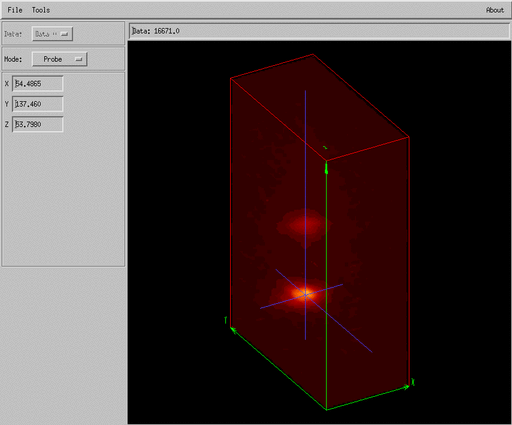
Slicer3 is a GUI widget based application to visualize three-dimensional data which comes with the IDL environment, a simple script to read an IFU data cube into the GUI is shown below,
here we create a pointer to our data array and pass this pointer to the slicer3 procedure. The Slicer3
GUI is shown in Figures 6 and 7. These display a projection of an IFU data cube and the user
operating on it with the cut and probe tools.
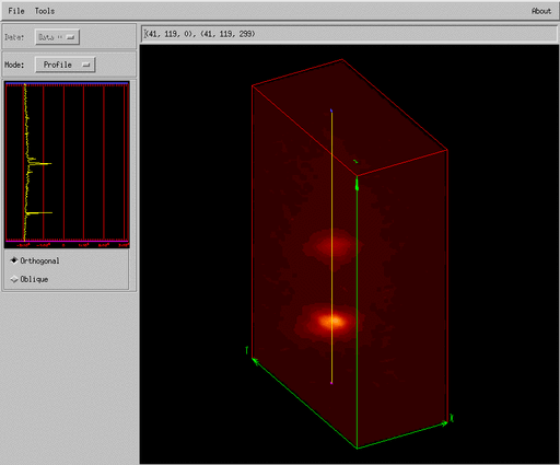
One of the interesting things about the Slicer3 GUI is that it is entirely implemented as an IDL procedure and the code can therefore be modified by the user for specific tasks. More information on Slicer3 can be found in the online help in IDL.
No discussion of astronomy data visualisation in IDL can be complete without reference to the IDL Astronomy Library. This IDL procedure library, which is maintained by the GSFC, provides most of the necessary tools to handle your data inside IDL. The library is quite extensive, and fairly well documented. A list of the library routines, broken down by task, can be found at http://idlastro.gsfc.nasa.gov/contents.html.
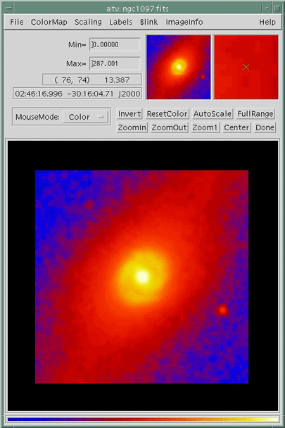
ATV is a frontend for the IDL tv procedure. Like the Slicer3 GUI discussed previously, ATV is entirely
implemented as an IDL procedure so it is simple to add new routines, buttons or menus if
additional functionality is needed. The interface, deliberately, resembles SAOimage so
that users can quickly start using it. Detailed usage instructions are available online at
http://www.physics.uci.edu/~barth/atv/instructions.html. However, to display an a plane in a
data cube you can pass an array directly to atv as follows.
Most of the packages we have discussed, e.g. Kappa, Figaro, and Ccdpack, are available from the IRAF command-line interface (up to the 2004 Spring release) and can be used just like normal IRAF applications (see SUN/217 for details) and IRAF CL scripts can be built around them as you would expect to allow you to analyse your IFU data cubes using their capabilities.
However, it should be noted that Starlink and IRAF applications use intrinsically different data
formats. When a Starlink application is run from the IRAF CL, the application will automatically
convert to and from the IRAF .imh format on input and output. This process should be transparent,
and you will only see native IRAF files. However, you should be aware, if you are used to using the
Starlink software, that the native NDF format is more capable than the IRAF format and some
information (such as quality and variance arrays) may be lost when running the Starlink software
from IRAF.
The scripts shipped within the Datacube package are described in SUN/237. The example dataset has a spectral axis in the wavelength system with units of Ångstrom, however Datacube can handle other spectral systems and units, as supported by the FITS standard.
You can make use of the Datacube squash shell script which is a user friendly interface to the Kappa collapse application allowing you to create both white-light and passband image, e.g.
Here we make a white-light image from the input data file ifu_file.sdf, saving it as a
two-dimensional NDF file out.sdf as well as plotting it in a GWM window (see Figure 9).
Alternatively we can make use of scripts command-line options and specify the input and output files,
along with the wavelength bounds, on the command line, as in this example.
Alternatively we can make direct use of the collapse application.
Here we collapse the cube along the third (λ) axis.
The Datacube package offers two ways to create passband images: first we may use (as before) the squash shell script, this time specify more restrictive λ limits, e.g.
would create a two-dimensional passband image, collapsing a 200 Å-wide section of the spectral axis.
Alternatively, we may choose to generate our passband image interactively using the passband shell script.
Here the script presents us with a white-light image and prompts us to click on it to select a good signal-to-noise spectrum, it then asks us whether or not we want to zoom in on a certain part of the spectrum. Let us zoom, and then the script allows us to interactively select a region to extract to create a passband image. It then plots this next to the white-light image for comparison.
Alternatively we can again we can make direct use of the collapse application, upon which both the squash and passband have been built, as shown below.
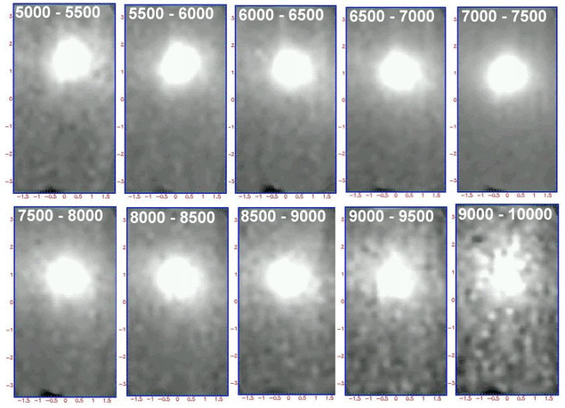
The Datacube package provides the step shell script to carry out this task.
Here we are asked for the lower and upper bounds of the desired wavelength range, and a step size. The script then generates a series of NDF two-dimensional passband images named chunk_*.sdf.
Alternatively, a very simplistic IDL script to step through an TEIFU data cube (stored in an NDF called
ifu_file.sdf) is shown below.
The script reads the NDF file in using the READ_NDF procedure, creates an IDL graphics window, and
steps through the data cube in the wavelength direction a pixel at a time.
There is now a Kappa command chanmap task that forms an image of abutting channels or passbands of
equal depth. It is also available from the cube toolbox in Gaia. Once created you may view the passband
image with Gaia or display. To read off the three-dimensional co-ordinates of features, in Gaia use
Image-Analysis→Change
Coordinates→Show
All Coordinates…, and in Kappa run cursor.
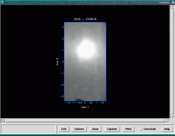
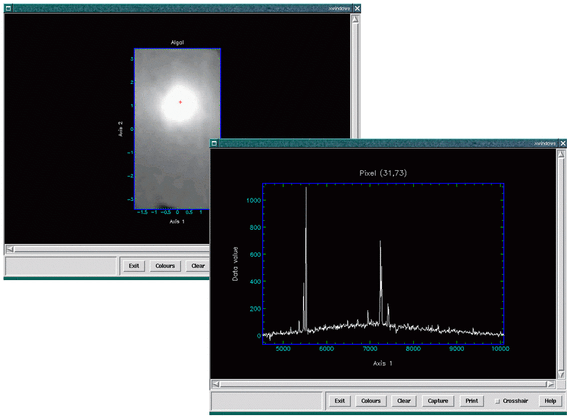
The ripper shell script in the Datacube package was designed as a user-friendly interface over the Kappa ndfcopy application.
Here we read in the data cube, ifu_file.sdf, and are prompted to click on a pixel to extract the
spectrum, see Figure 12.
Alternatively we can use ndfcopy directly as underneath.
Here we extract the same spectrum by using NDF sections to specify a region of interest,
and the TRIM and TRIMWCS parameters to reduce the dimensionality of the file to only one
dimension.
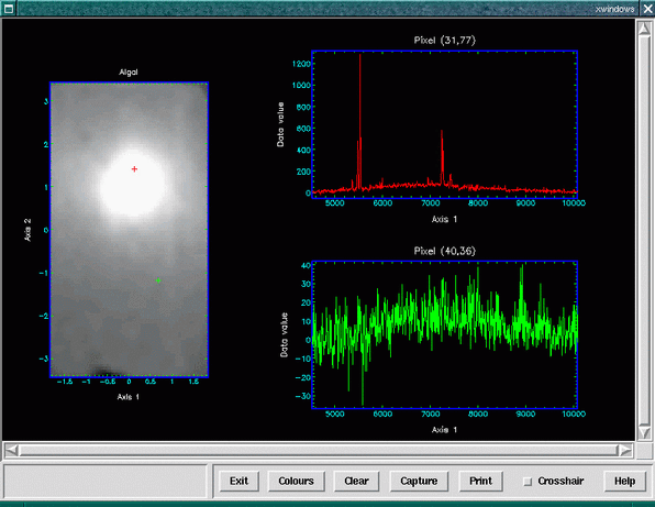
The compare script was written to give you this capability. It allows you to continually select spectra from different parts of the cube, plotting the two most recent to the right of a white-light image of the cube. See Figure 13.
For instance,
Here the script presents us with a white-light image and asks us to click on a pixel. It then extracts and displays the spectral axis associated with that pixel in the upper right of the display window. We then have the opportunity to select another pixel, the corresponding spectrum being displayed in the lower right of the display window. We extract only two spectra during this run of the script (Figure 13), pressing the right-hand mouse button to terminate. However, if we carried on and selected a further spectrum it would replace our original in the upper-right panel of the display window. Selecting a further spectrum would replace the lower-right panel. The location of each new spectrum plot alternates.
Also see how Gaiacompares spectra Section 5.5.2.
The Datacube package provides two tasks to carry out this process, the stacker (see Figure 14) and multistack shell scripts.
A run of the stacker script is shown below.
Here we extract three spectra by clicking on a white-light image of the data cube, and these are then plotted with an offset of 200 counts between each spectrum. We then get the opportunity to zoom into a region of interest, and the three spectra are then re-plotted.
The multistack script operates in a similar manner, however, here we are prompted for the number of spectral groups required, and the number of spectra in each group. The mean spectrum of for each ‘group’ of spectra is calculated, and then all the mean spectra are plotted in a stack as before, as seen in the following example.
Here we request three groups of four spectra each, i.e. we’ll get three mean spectra plotted as a stack in the final display.
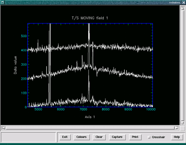
For an overview visual inspection of the spectra in a cube, it is useful to plot many spectra
simultaneously, albeit at a lower resolution, in their respective spatial locations. While
Kappa provides the clinplot command to make such a grid, sometimes the sheer number of spatial
pixels can make the spectra unreadable and will take some time to plot. Therefore the
Datacube package offers the gridspec shell script. It has an option to average the spectra
in the spatial domain, thereby reducing the number of spectra plotted by several times,
generating more practical graphics quicker. See Figure 15. Below is an example. The -z option
requests that the white-light image be shown and a subset of the cube selected with the
cursor. The -b option sets the spatial blocking factor. Different factors may be given for
x and
y, the
two values separated by a comma.
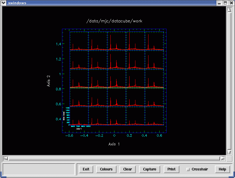
A useful strategy is to select a blocking factor that gives no more than ten plots2 along an axis. Then focus on regions of interest—you either supply an NDF section or select from the white-light image—by decreasing the blocking, and thus increasing both the spatial and spectral plotting resolutions.
The Datacube package provides the velmap and velmoment shell scripts to manage this fairly complex task. velmap fits Gaussians to a selected line, and involves some graphical interaction to select the template spectrum, and initial fitting parameters. For data well characterised by a Gaussian, velmap can produce excellent results. However, it is an expensive algorithm to apply to each spatial pixel. Also Gaussian fitting is not appropriate for all data.
The alternative offered velmoment collapses along the spectral axis by deriving the
intensity-weighted mean co-ordinate, and converts this to a velocity. This is turbo-charged compared
with fitting. The downside is that the results will not be as accurate as line fitting, and care
must be taken to select regions of the spectra populated by a single significant emission
line.
By fitting
velmap allows you to select the highest signal-to-noise spectrum from a white-light image. You can
then interactively fit a line in this spectrum. The script will attempt to automatically fit the same line in
all the remaining spectra in the cube, calculate the Doppler velocity of this line from a rest-frame
co-ordinate you provide or is read from the NDF WCS, and create a velocity map of that line in the
cube. See Figure 16. Below is an example.
As no automatic process is ever perfect the script allows you to manually refit
spectra where it had difficulties in obtaining a fit. If the script was unable to fit an
(x,y)
position this value will be marked as VAL__BADD in the final velocity map. Should you choose to Refit
points, clicking on these (normally black) data points in the final output image will drop you into an
interactive fitting routine. However, you are not restricted to just refitting those points where the
script was unable to obtain a fit, you may manually refit any data point in the velocity
map.
There is a -a option where you can review each fit at each spatial pixel. The fit parameters can be
logged to a Small Text List with the -l option.
By moments
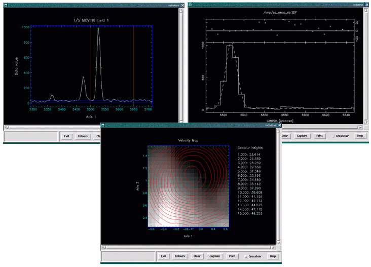
The second script for generating a velocity map is velmoment. This first allows you to select a region
of interest. For large regions or noisy spectra you can also request spatial averaging (-b option) to
reduce the spatial dimensions by integer factors. If your dataset has a WCS SPECTRUM or
DSBSPECTRUM Domain, velmoment then switches co-ordinate system to one of four
velocities, such as optical or radio. It can also cope with NDFs in the UK data-cube format
too.
Then comes the heart of the script—the collapse task acting upon the spectral axis. It derives the
intensity-weighted velocity moment. For simple spectra, i.e. a single or dominant emission line,
collapse finds a representative velocity for the line.
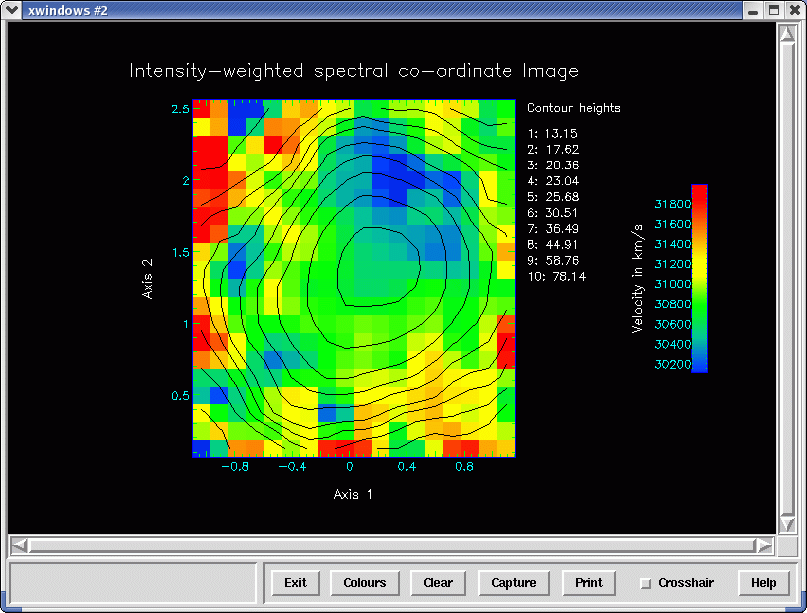
The final stage is to display the map of the velocities. It uses a colour table that runs from blue to red
in order to give a visual clue of the relative motions. You may choose to superimpose optional
contours of the white-light image upon the velocity map.
Here is an example. Rather than supply a spatial subset as in the velmap
example, we choose to select the spatial region for analysis by interacting with a
2×2
spatially averaged (-b 2) ‘white-light’ image that the script presents. The wavelength bounds in the
NDF section 5300.:5750. restricts the spectral compression to the range 5300 to 5750 Ångstrom and
brackets the [OIII] line. This means that the ’white-light’ image is effectively a map of the [OIII]
emission. The script converts the intensity-weighted wavelengths into velocities that it displays with a
key and suitable colour map. Finally it overlays a ten-level contour plot of [OIII] map on the velocity
map. See Figure 17. Below is an example.
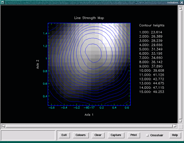
The Datacube peakmap script will generate a line-strength map. The interface to this script is very similar to that of the velmap script discussed in Section 5.8.8, and it also generates final output in a similar form, see Figure 18. Much like the velmap script the peakmap script allows you to manually refit any spectrum that you think may have been poorly fitted by the automatic process.
It should be noted that generating a passband image of a line region, and a line-strength map using the peakmap script, should yield similar results. If you are worried about how accurately the automatic fitting of gaussians is doing on a particularly noisy image, then generating a line-strength map and making this comparison is an easy way of deciding a level of trust in your velocity maps, as these are generated using the same fitting algorithms.
No, neither peakmap nor velmap handle multiple gaussians or blended lines. While the
Figaro fitgauss application on which these scripts are based can handle fitting blended lines—up to
six through the NCOMP parameter—automating this process reliably proved to be extremely difficult
and made the fitting routine very fragile to signal-to-noise problems.
Make a line-strength map of the both lines using peakmap or passband images using squash, and then use the Kappa div task to divide one by the other to create a ratio map. Here is an example.
Mosaicking IFU data cubes poses unique problems. Firstly the field of view of all the current generation of instruments can be measured in arcseconds, far too small for the traditional approach of image registration to allow the cubes to be matched up the x,y plane, additionally, the wavelength calibration of the two cubes you wish to mosaic may be entirely different, certainly the case for cubes coming from different instruments.
Unfortunately mosaicking therefore relies critically on WCS information provided in the cube FITS headers. Currently the form this information takes varies between cubes from different instruments; and sometimes where active development work is ongoing, between different cubes produced by the same instrument. It is therefore very difficult to provide a ‘catch all’ script or even recipe to allow you to mosaic two cubes together as yet. The agreement of a standard for the spectroscopic world co-ordinates promulgated in FITS (Greisen et al., 2006, Representations of spectral coordinates in FITS, Astronomy & Astrophysics 446,747) should diminish the problem. At the time of writing the Starlink AST already supports spectral frames (these are used to compute the velocities in velmap), and most features of this FITS standard.
If the data cubes to be combined have valid WCS information, you should try the wcsmosaic task. If your spectral co-ordinates are only present in an AXIS component, see the section Converting an AXIS structure to a SpecFrame in SUN/95.
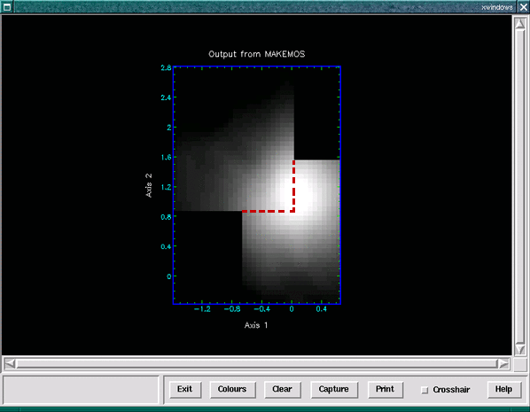
Without valid WCS information we offer a possible approach to the problem. If the two data cubes have identical spectral-axis, e.g. wavelength, calibrations and, rather critically, the same number of pixels along the spectral axis, (i.e. they are from the same instrument); then the approach we take to the problem is to determine the right ascension and declination of the centre of the x,y plane and work out the offset between the two frames in pixels. You can probably use the AXIS frame to determine the arcsecond-to-pixel conversion factor, or this may be present in the FITS headers.
Then make use of the Ccdpack wcsedit application to modify the origin of the PIXEL frame of one of the cubes such that the two cubes are aligned in the PIXEL frame. Next we suggest you change the current frame to the PIXEL frame (with wcsframe) and use makemos to mosaic the cubes together (see Figure 19). It should be noted that makemos pays no attention to the WCS information in the third axis (being designed for two-dimensional CCD frames) which is why having an identical wavelength calibration over the same number of pixels is rather crucial.
Alternatively use can be made of the Ccdpack wcsreg application to align the cubes spatially.
Due to the differences in WCS content between instruments, if you want to mosaic cubes from two different instruments together, the only additional advice we can currently offer you is that you should carefully inspect the WCS information provided by the two cubes using (for instance) wcsedit and try to find a way to map a frame in the first cube to a frame in the second. It may then prove necessary to re-sample one of the cubes to provide a similar wavelength scale. This may involve using Kappa tasks wcsadd to define a mapping between frames, and regrid to resample.
1/star/etc/ is for a standard Starlink installation, but the Starlink software may be in a different directory tree on your
system.
2This is a guide figure. The limit will depend on your hardware and the size of your plotting window. It will be more for a higher-resolution hardcopy.